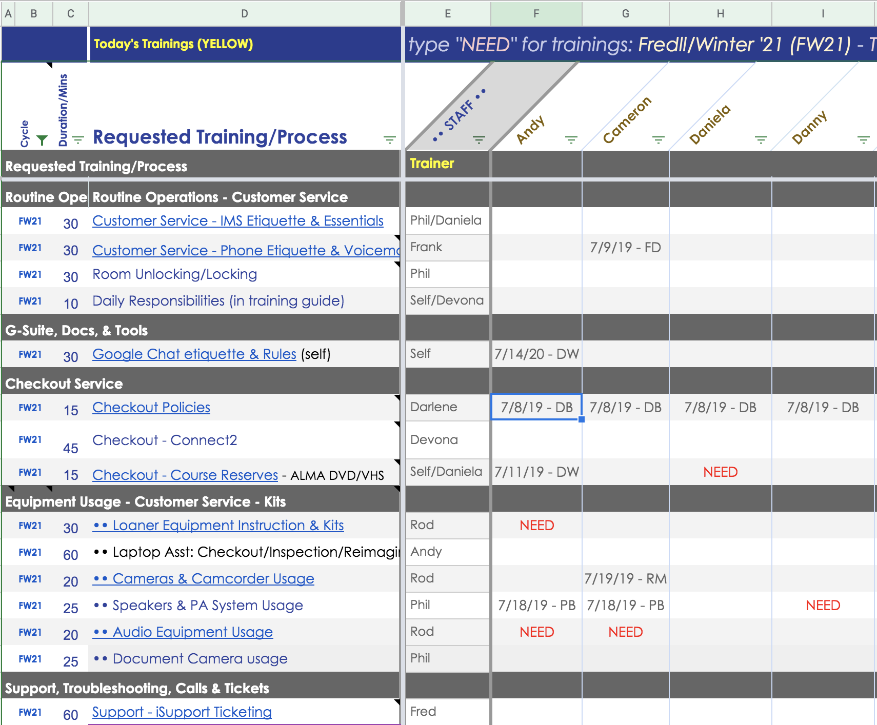
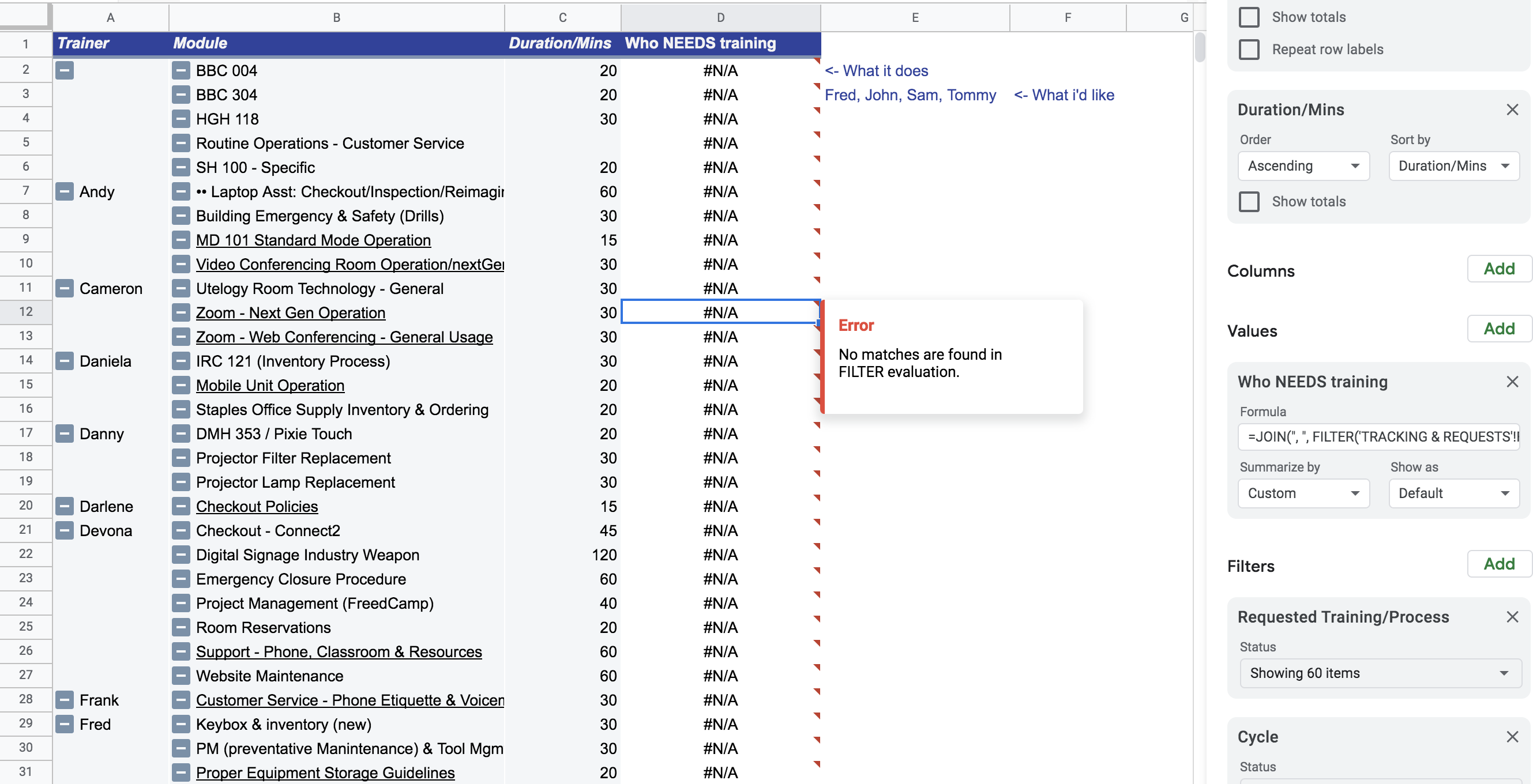
In an effort to organize staff training: So far I've made the pivot table, but I'd like for the pivot table to extract who needs which training, as a list in one cell. I tried using =JOIN, but I have no idea what else.
On sheet 1:
- Row 2: Staff (who need the training), They enter "NEED" in the row of the column for that training.
- Column D: The Names of Trainings
- Column E:Trainers Trainers/Staff who are providing the training

On Pivot Table
Columns
- A: Trainer
- B: What modules they're teaching
- C: How long the training is
- D: A cell that lists who requested the training (who entered "NEED" into Sheet 1)
I'm trying to tell it simply:
- Look for the name of THIS training over in sheet 1, AND if the value of a cell in that row is "NEED", Return the Name of person/people and list it in one cell next to this pivot table......(lollll I will not cry).
The formula would be something like:
Pull the name of the people from Sheet1!F1:Z if (Training names) Sheet1!D:D match Pivot table B:B AND there's a "NEED" in the row of that training....then list those names in ONE CELL.
I'm over explaining I think, but this has taken all day and my brain simply cannot any longer and my own formulas sheet is not helping, Please help if you can.
I have tried: =JOIN mixed with Match, then Filter... Idk what i'm doing. And the pivot table has no option to filter "NEEDS" from the whole data set. Instead it makes me filter the "NEEDS" of a Name/Column, but if i do that, it will filter out everyone elses data. Basically it forces me to make a custom formula, which is great because I can learn, but... I really hope all of this made sense :(. Any help would be heavenly.

