1

I have a couple of datasets with the same columns entered horizontally next to each other.

I have a data / facebook leads / facebook adspend column for thee moonth of january in column a, b, c and the same columns for the mounth of february in column e, f, g (but in a different order). What I want is to merge the data of both months vertically: So only have one dat / facebook leads / facebok adspend column.

So I want to automatically merge the data of all columns that have the same labels / headers vertically.

The problem is that is a quite large dataset and the columns are not in the same order and also it's dynamic, so each month there's a new set of data entered in the sheet. So I can't do it with a query formular, where I have to pick each array manually. What I'm looking for is a formula, that "scans" an the whole sheet, "find" the columns with a certain name and merges them vertically.

Here's the dataset: https://docs.google.com/spreadsheets/d/1DkPmrmDTpEGGD9wvpv1Z8uq0ge-YwHrbcG3WP4vi3aY/edit#gid=2100307022

2
  • 1
    your link goes nowhere
    – Blindspots
    Commented Dec 30, 2022 at 0:43
  • sorry, now it works Commented Dec 30, 2022 at 8:33

1 Answer 1

1

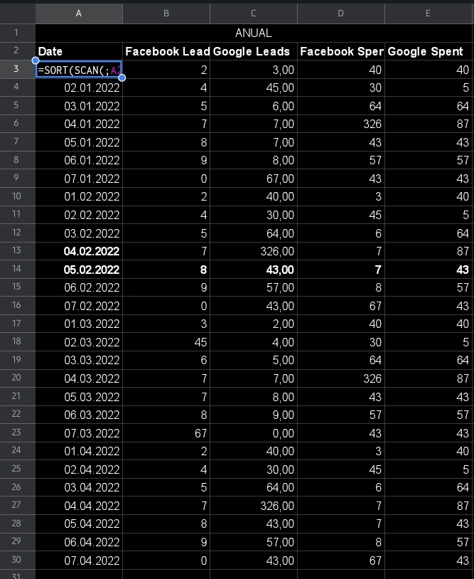
I've created a new sheet with the raw data and another with my possible solution. See if it's useful:

=SORT(SCAN(;A2:E2;LAMBDA(ag;va;{FLATTEN(FILTER('Raw Data'!A3:Z1000;'Raw Data'!A2:Z2=va))})))

enter image description here

Some latter clarifications for who may read this in the future:

in order for this to work and the rows be correctly alligned,you'll need to always have those 5 headers each time a new set of columns if added. If by chance some time it doesn't, include it or the sorting will be messed up. 2) In order to include more columns, if you know that the rows won't be that much (you can change the ranges to include all further columns: =SORT(SCAN(;A2:E2;LAMBDA(ag;va;{FLATTEN(FILTER('Raw Data'!A4:100;'Raw Data'!A2:2=va))}))) Just change 100 with some bigger or smaller number of your convenience. (Or insert new columns in between the existing range and not at the end, obviously that would work too)

8
  • thank you so much, this helps a lot!! The only thing is, that I don't quite understand it. Would you mind explaining it a little bit? I know it's probably a lot to ask, but it would really help me using it further. Commented Dec 30, 2022 at 12:17
  • No problem: SCAN let me perform the same operation through the five headers of A2:E2 one by one (LAMBDA is just auxiliary of it for naming variables) I use FILTER to find the columns that match the headers, FLATTEN to join all those found columns in one. And finally I use SORT because FLATTEN would have the values mixed by its original rows. Let me know if it's helpful!
    – Martín
    Commented Dec 30, 2022 at 12:39
  • ok this was very helpful Commented Dec 30, 2022 at 13:28
  • still have a couple of questions if it's ok: =SORT(SCAN(;A2:E2;LAMBDA(ag;va;{FLATTEN(FILTER('Raw Data'!A3:Z1000;'Raw Data'!A2:Z2=va))}))) ag = is this the name of the lambda function? va = is actually a variable to store A2:E2? SCAN(**;**A2:E2 = the first semicolumn confuses me a bit (in the formula description it says that the first argument is the "first value" - but you don't need that in this case so you just leave it empty, correct? Commented Dec 30, 2022 at 13:36
  • Right, it's a kind of "trick". SCAN is used for partial or accumulative calculations and sequences, for example. But by not using that argument it allows me to have the five independent columns in just one formula, that won't be possible with the limitations of another ARRAYFORMULAs
    – Martín
    Commented Dec 30, 2022 at 13:48

Your Answer

By clicking “Post Your Answer”, you agree to our terms of service and acknowledge you have read our privacy policy.

Not the answer you're looking for? Browse other questions tagged or ask your own question.