2

I have a simple table with columns:

  • A (Donor ID)
  • B (Donation date)
  • C (Donation Amount)

I need to extract the following report:

For each donor ID most recent donation date and amount donated corresponding to that date. I have tried several Query and Filter function but does not seem to work.

2 Answers 2

2

Wilson. Here is another approach (assuming the date is in A1:C):

=ArrayFormula(IFERROR(VLOOKUP(UNIQUE(A:A),QUERY(A:C,"Select * Order By B Desc",1),{1, 2, 3},FALSE)))

Just be sure to format the resulting date column as dates, since by default is will use the raw number format of the data (i.e., the number of days since December 30, 1899, which will be numbers in the mid-40,000 range).

HOW IT WORKS:

Essentially, we form a virtual range of just the UNIQUE donors (as well as the header) with UNIQUE(A:A). (This will also include one blank, since that would be unique in the column one time.)

We VLOOKUP only those values in another virtual range: a QUERY of the A:C data upside-down by date (i.e., with the most recent dates always on top). By looking up only unique donors and the header from A in this upside-down range, the first match found will always be their most recent donation.

We return columns 1, 2 and 3 from this upside-down QUERY range (i.e., the three points of data, and the headers).

FALSE tells Google Sheets that the virtual range is not in order by the key column (Donor) and instructs it therefore to look for exact matches only.

The IFERROR wrapping on the VLOOKUP prevents the formula from trying to return a result for that UNIQUE blank I mentioned.

3
  • looks like this approach cant handle IDs which are fully numeric unless whole column A is formatted as text. also, wrapping query into to_text() can fix the date formatting issue
    – user0
    Commented Jan 28, 2019 at 0:42
  • @MARK, I haven't seen the OPs actual data. I would assume that all IDs are all of the same type (i.e., either all numbers or all text) and that all dates are actual dates. What causes you to think this isn't the case? Did I miss a link to the OPs data that may have been removed? Or did you get special permission to access his sheet?
    – Erik Tyler
    Commented Jan 28, 2019 at 3:03
  • @MARK, yes you have mixed data in Column A: text and numbers. Proper data controls in an actual sheet of serial numbers would either all be text or all be numbers. QUERY requires one or the other; if there is a mix, text will come in as blanks. But this could easily be controlled for in the QUERY range call if needed.
    – Erik Tyler
    Commented Jan 28, 2019 at 4:12
-1

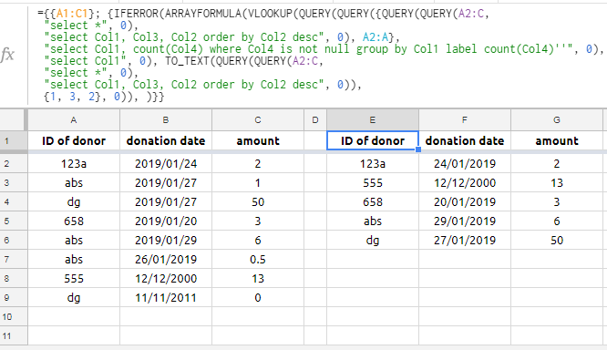
={{A1:C1}; {IFERROR(ARRAYFORMULA(VLOOKUP(QUERY(QUERY({QUERY(QUERY(A2:C,
  "select *", 0),
  "select Col1, Col3, Col2 order by Col2 desc", 0), A2:A},
  "select Col1, count(Col4) where Col4 is not null group by Col1 label count(Col4)''", 0),
  "select Col1", 0), TO_TEXT(QUERY(QUERY(A2:C,
  "select *", 0),
  "select Col1, Col3, Col2 order by Col2 desc", 0)),
  {1, 3, 2}, 0)), )}}

enter image description here

Your Answer

By clicking “Post Your Answer”, you agree to our terms of service and acknowledge you have read our privacy policy.

Not the answer you're looking for? Browse other questions tagged or ask your own question.