0

Ive got a Pivot table in a Google Sheet which summarises some numerical data by groups.

Ive attached a screenshot of the pivot table below.

I want to be able to sum the values of the "grand total" in B and C. eg =sum(b7:c7) which i can do, but as soon as another element is added to the raw data or a filter is applied to the pivot table the grand total row moves and my sum formula breaks.

Is there a way i can "anchor" my forumla to the grand total values, something like this pseudo code : sum($grand_total_of_Frequency : $grand_total_of_Qty)

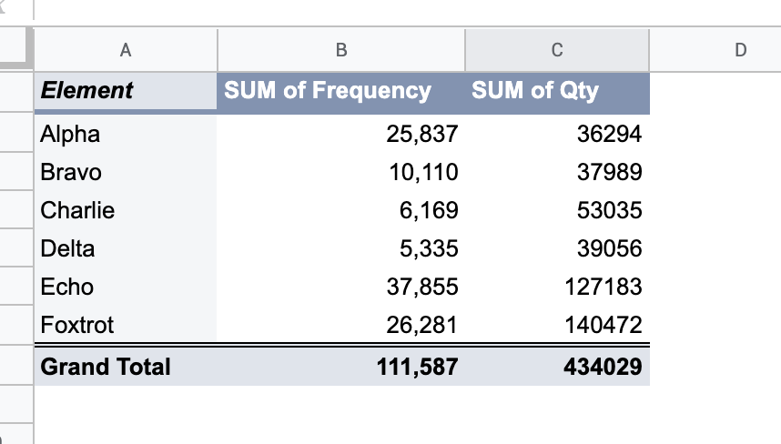
screenshot of pivot table

2 Answers 2

1

You could use a QUERY formula combined with the SUM function:

=sum(QUERY(A1:C11,"select sum(B), sum(C) where A<>'Grand Total'"))

What you actually do is to recreate and sum the sums from the Pivot Table itself, omitting the values of the Grand Total.

You can place the formula wherever you like.

0

You can add a "Calculated field" which sums Frequency and Qty, you will get a sum for every element with its respective Grand Total

Your Answer

By clicking “Post Your Answer”, you agree to our terms of service and acknowledge you have read our privacy policy.

Not the answer you're looking for? Browse other questions tagged or ask your own question.