Multiple Gsheets data querys

Question

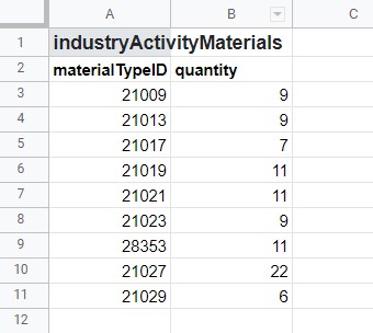
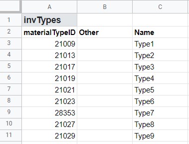
Hey all so I currently have 3 Gsheets. 2 are sql imports with the below tables. The goal is to get the information based off a Type Id 28353 into my Master sheet. The plan is to get all values from one of the tables that match the Type ID I have. I then want to be able to take the value in col1 and replace it with the correct name instead of the number. =query(importrange(xls_url!B1,"industryActivityMaterials!A1:D40000"),"select Col3, Col4 where Col1 matches '"&B1&"'") This first query will respond with the below query

materialTypeID  quantity
21009   9
21013   9
21017   7
21019   11
21021   11
21023   9
21025   11
21027   22
21029   6

I know that the names can be queryed with this next query =VLOOKUP(A17,importrange(xls_url!B$2,"invTypes!A2:C"),3,false) . The question is How can I combine the Two query's so that the MaterialTypeID will have the expected name returned from query 2 ?

Another question With the First query can I prevent the response of materialTypeID quantity ? These values do reside at row 1 of the first sheet?

Answer 1

Try this in the "Master" spreadsheet file:

=query({query({importrange(B3,"A2:C")},"select Col1,Col3 where Col1 contains '" &B4&"'",0),query({importrange(B2,"A2:B")},"select Col2 where Col1 contains '" &B4&"'",0)},"select Col1, Col3, Col2")

• Enter the Spreadsheet URL for "industryActivityMaterials" in cell B2
• Enter the Spreadsheet URL for "invTypes" in cell B3
• Enter the "materialTypeID" that you want to query in cell B4

Logic

• the query consists of two nested queries.
• Both of the nested queries use importrange to access data the external spreadsheets.
  • each nested query includes a where clause: Col1 contains '" &B4&"'"
    • this returns only the records that contain the "materialTypeID" entered in Cell B4. For the purposes of this answer, it is assumed that each spreadsheet contains only one record per ID.
• the output of the nested queries are combined in the range of single query using curly brackets {} and separated by a comma (for countries that use decimal point notation).

---

Master

---

Spreadsheet: industryActivityMaterials

---

Spreadsheet: invTypes