How can I set conditional formatting on a particular cell that depends on another cell's value?

Question

In my example I would like to conditionally format column B cells. Those marked with x should be formatted according to value in column A (in the example the value is 1):

A | B
1 | x
2 | 
3 | 
1 | x
1 | x
4 | 
8 |

// x can be any value and is here merely to mark the cell that should be formatted

IMPORTANT 2014 NOTE: Conditional formatting based on formula that may include other cells is now possible in Google Sheets, and works very similarly to how Excel spreadsheets work. This answer explains its use.

Answer 1

Complex conditional formatting can be achieved in Google Spreadsheets using Google Apps Script. For example, you could write a function that changes the background colour of an entire row based on the value in one of its cells, something that I do not think is possible with the "Change color with rules" menu. You would probably want to set triggers for this function such as "On Edit", "On Open" and "On Form Submit".

Documentation for setBackgroundRGB() function

UPDATE: Here is a Google Apps Script example of changing the background color of an entire row based on the value in column A. If the value is positive, use green. If empty, white. Otherwise, red. See the results in this public Google Spreadsheet. (You will have to be signed in for the script to run, but without signing in you can still see results).

function colorAll() {
  var sheet = SpreadsheetApp.getActiveSheet();
  var startRow = 2;
  var endRow = sheet.getLastRow();

  for (var r = startRow; r <= endRow; r++) {
    colorRow(r);
  }
}

function colorRow(r){
  var sheet = SpreadsheetApp.getActiveSheet();
  var dataRange = sheet.getRange(r, 1, 1, 3);

  var data = dataRange.getValues();
  var row = data[0];

  if(row[0] === ""){
    dataRange.setBackgroundRGB(255, 255, 255);
  }else if(row[0] > 0){
    dataRange.setBackgroundRGB(192, 255, 192);
  }else{
    dataRange.setBackgroundRGB(255, 192, 192);
  }

  SpreadsheetApp.flush(); 
}

function onEdit(event)
{
  var r = event.source.getActiveRange().getRowIndex();
  if (r >= 2) {
    colorRow(r);
  }
}

function onOpen(){
  colorAll();
}

​

Answer 2

The new Google Sheets allows you to do this, as described here. You have to first enable the new spreadsheets in your Google Driver settings as described in the article. Then you can select 'Custom formula is' from the conditional formatting options and enter any formula (do not forget to add the = prefix!). Cell references without $ prefixes are adjusted automatically when applied to ranges as you would expect.

It seems that support for migration from old to new is lacking - it only applies to new sheets and I found that only values could be copied from one to the other. Copying an entire sheet may be an option.

Answer 3

Google Sheets' Conditional format rules look like this if you want to conditionally format with a red background if the sum in two cells is different than in 3rd cell:

Answer 4

Conditional formatting - custom formula

range 2:227

= if($i:$i = "Duplicate",True,False)

select the color you want the row to be highlighted.

Answer 5

(Feb 2017) As mentioned in another answer, Google Sheets now allows users to add Conditional Formatting directly from the user interface, whether it's on a desktop/laptop, Android or iOS devices. However, the rest of this answer is primarily for developers because you can write apps "do" conditional formatting.

With the Google Sheets API v4 (and newer), developers can now write applications that CRUD conditional formatting rules. Check out the guide and samples pages for more details as well as the reference docs (search for {add,update,delete}ConditionalFormatRule). The guide features this Python snippet (assuming a file ID of SHEET_ID and SHEETS as the API service endpoint):

myRange = {
    'sheetId': 0,
    'startRowIndex': 1,
    'endRowIndex': 11,
    'startColumnIndex': 0,
    'endColumnIndex': 4,
}

reqs = [
    {'addConditionalFormatRule': {
        'index': 0,
        'rule': {
            'ranges': [ myRange ],
            'booleanRule': {
                'format': {'textFormat': {'foregroundColor': {'red': 0.8}}}
                'condition': {
                    'type': 'CUSTOM_FORMULA',
                    'values':
                        [{'userEnteredValue': '=GT($D2,median($D$2:$D$11))'}]
                },
            },
        },
    }},
    {'addConditionalFormatRule': {
        'index': 0,
        'rule': {
            'ranges': [ myRange ],
            'booleanRule': {
                'format': {
                    'backgroundColor': {'red': 1, 'green': 0.4, 'blue': 0.4}
                },
                'condition': {
                    'type': 'CUSTOM_FORMULA',
                    'values':
                        [{'userEnteredValue': '=LT($D2,median($D$2:$D$11))'}]
                },
            },
        },
    }},
]

SHEETS.spreadsheets().batchUpdate(spreadsheetId=SHEET_ID,
        body={'requests': reqs}).execute()

In addition to Python, Google APIs support a variety of languages, so you have options. Anyway, that code sample formats a Sheet (see image below) such that those younger than the median age are highlighted in light red while those over the median have their data colored in red font.

NOTE: my answer here is identical to the one over on SO for this question except I dropped the PSA as it doesn't need to live in >1 place.

Answer 6

To address the specifics of the Q in 'new' Sheets, I suggest clearing any conditional formatting from B:B, selecting ColumnB and applying a Custom formula is of:

=A1=1

with formatting of choice and Done.

Answer 7

When editing conditional formatting, select Custom formula and use the following...

=if(A1 = 1 , true)

Select your colors and you are done.

Answer 8

Edit in response to the question's clarification:

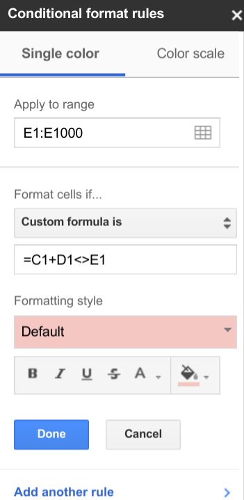
In your Google Spreadsheet window, there is a menu Format with the option "Change color with rules". This is as technical as Google Spreadsheet's conditional formatting is. As far as I can tell, there is no way to color one cell based on another's value - Google doesn't let you enter formulas for other cells.

Unless you're putting other data into column B, you could always make all of column B equal column A, and then use the "Change color with rules" option to color all the cells with the value of 1 with like colors - ie, red background and red text when the value is 1, white background and white text when it is not, effectively hiding the value in column B. That will give you the look you want.

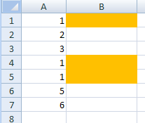
In Excel, you can do what you want. Using your data as an example, I conditionally formatted B1 when this formula is true:

=IF(A1=1,true,false)

and then dragged the formatting down, which highlighted only the cells in B where it's a neighbour in column A equalled 1.

---

Original Answer

I'm not sure if you can do this in 2 columns, but I know you can do it in 3:

 A  |  B  |  C
----------------
 1  |  f  |  x

In the B column, you can use the IF formula to see whether an x has been placed in the appropriate C column:

=IF(C1="x",A1,"") 

The IF formula has 3 parts - the test, the then value, and the else value. In the above example, the formula checks to see if there is an x in the C column. If there is, it enters the value from A1, otherwise, it enters a blank. It doesn't matter if the x is upper- or lower-case.

Once you enter this formula at the top of your list, you can use the drag feature to drag the formula down for the rest of your list. With the cell highlighted in blue, move your mouse over the square in the lower right corner until the cursor becomes a crosshair. Then just click and hold while dragging down to copy the formula to the cells below.