Add hourly rate to line items based on line item date

Question

Hello, I'm trying to set up a system using google forms and google sheets to keep track and analyse my business's employee's hrs and wage.

My idea is:

Use a simple Google Form to for employees to submit their daily hrs. (The Name will be a dynamic list using the Form Ranger Addon which will be populated by a google sheet which has a list of all employees names.)

The Google Form will be linked to this Google Sheet which holds the columns Employee | Date | Start time | End time and then the calculated columns Total Hrs and Hourly Rate.

This is where I get stuck! ​ I want the Hourly Rate to be an arrayformula and to be dynamic based on the values of a different sheet. Let me explain!

Employee wages might change throughout the year and I would like the hourly rate line amount accounting to each employees daily submission to be dynamic based on the employees changing rates.

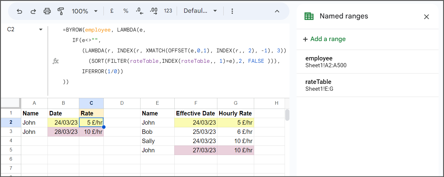
I thought to have a separate sheet where I will fill in employees hourly rate and every time the rate changes. This will look like this.

So finally:

How do i write an array formula that returns the employees hourly rate based on the date in the row (output of daily from submission)?

I was thinking some kind of nested XLOOKUP but I'm totally stuck.

Help please good people! :D

Google Form and Google Sheet

Answer 1

Formula

This formula will return the hourly rate based on the date worked ignoring future increases that do not apply.

=LAMBDA(r, INDEX(r, XMATCH(dateWorked, INDEX(r,, 2), -1), 3))
 (SORT(FILTER(rateTable,INDEX(rateTable,, 1)=employee),2, FALSE ))

Conditions

• "dateWorked" is the day the hours are worked (in form);
• "rateTable" is a 3 column range with
  1. employee names in column 1;
  2. dates in column 2 (effective date for the new hourly rate);
  3. hourly rates in column 3
• "employee" is the employee name (in form)

Notes

1. LAMBDA is used to avoid repeating the initial SORT and FILTER and use r in its place
2. "rateTable" is filtered for the employee and then sorted in descending order by date: r
3. XMATCH is used to find the date in r that either matches the date worked or is older.
4. INDEX returns the hourly rate in the same row as the XMATCH-ed date

BYROW Version (single formula)

This version takes the formula above and uses BYROW to perform the same LAMBDA formula for each row in the name column (column A).

• a named range employee was created A2:A500,
• BYROW passes each row employee into a LAMBDA function where the current row is represented by the arbitrarily chosen name e
• If e is empty (no data entered) the formula is skipped: IF(e<>"", <formula>, IFERROR(1/0) (`IFERROR(1/0) is a sheets trick to return a genuinely blank result) ;
• to get the "employee" from the current row (e.g. A2) I can now use the e in the formula;
• for the "dateWorked" in the formula I can use the same e variable but use OFFSET to indicate where the data is located in relation to "employee". In this "dateWorked" is 0 rows and 1 column away from the "employee" column: OFFSET(e, 0 , 1) `

=BYROW(employee, LAMBDA(e, 
   IF(e<>"", 
      (LAMBDA(r, INDEX(r, XMATCH(OFFSET(e,0,1), INDEX(r,, 2), -1), 3))
        (SORT(FILTER(rateTable,INDEX(rateTable,, 1)=e),2, FALSE ))),
      IFERROR(1/0))
))