0

I have Google Sheets running the add-on Form Mule to automatically send emails with the responses to a Google Form. Using the following formula, I was able to get a nice HTML table to show up in the body of each email.

=RANGETOTABLE(FILTER(D:AH,A:A=A2),$D$1:$AH$1)

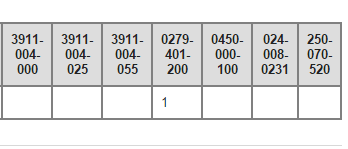
This returns a table that looks like this:

Blank cells and a single response cell

I want to try and filter the cells with nothing in them, out, so that only cells with values in them are returned.

1
  • Now the question doesn't make sense. If you selectively drop cells from each row, that's not a table anymore.
    – user79865
    Commented Jul 28, 2016 at 19:09

2 Answers 2

2

You can include multiple conditions in a filter by using multiplication (which means logical AND). For example,

FILTER(D:AH, (A:A=A2) * LEN(E:E) * LEN(H:H))

requires A to be equal to A2 and E to be nonempty and H to be nonempty.

Conditions can also be combined using addition, which stands for logical OR:

FILTER(D:AH, (A:A=A2) * (LEN(E:E) + LEN(H:H)))

requires A to be equal to A2 and that either E or H be nonempty.

If you have a lot of columns (like D:AH), one of which must be nonempty, the formula will have to be somewhat long. Instead of adding lengths as above, one can use concatenation & to shorten it a bit:

FILTER(D:AH, (A:A=A2) * LEN(E:E & F:F & G:G & H:H & I:I & J:J & K:K & L:L & M:M & N:N & O:O & P:P & Q:Q & R:R & S:S & T:T & U:U & V:V & W:W & X:X & Y:Y & Z:Z & AA:AA & AB:AB & AC:AC & AD:AD & AE:AE & AF:AF & AG:AG & AH:AH))`

Long, but you only have to do it once.


By the way, I used a spreadsheet to generate the long string above, by making a column of letters (say, in A1:A30) and then using =join(" & ", arrayformula(A1:A30 & ":" & A1:A30)))

6
  • So could I just do: =RANGETOTABLE(FILTER(D:AH,A:A=A2 * LEN(D:AH)),$D$1:$AH$1) in order to only return responses that are non-empty? Did I place it correctly? Commented Jul 28, 2016 at 17:47
  • Unfortunately, LEN won't work with a two-dimensional array like that. See my edit.
    – user79865
    Commented Jul 28, 2016 at 18:06
  • To isolate the problem, try the FILTER formula on its own, without Rangetotable.
    – user79865
    Commented Jul 28, 2016 at 18:23
  • Since I know D1:AH1 will always have something (as they are the headers) I only really need it to return a result when D2:AH2 have responses. But it is possible then to remove the column altogether without jacking up the ordering? Commented Jul 28, 2016 at 18:29
  • 1
    The filter removes the rows not columns. A row is dropped if all of the cells D-AH in that row are empty. If this is not what you wanted, edit the question with a more specific explanation of what you want.
    – user79865
    Commented Jul 28, 2016 at 18:31
0

You can include in your formula something like A:A<>"" that way it will ignore values in column A that are blank.

So: =RANGETOTABLE(FILTER(D:AH,A:A=A2,A:A<>""),$D$1:$AH$1)

Your Answer

By clicking “Post Your Answer”, you agree to our terms of service and acknowledge you have read our privacy policy.

Not the answer you're looking for? Browse other questions tagged or ask your own question.