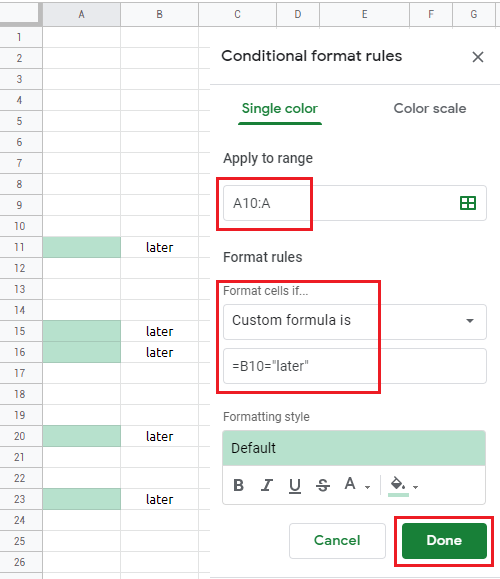
I want to use Conditional formatting so all of the cells in column A change colors whenever the matching cells in column B have the word "later".
ex: If cell B20 contains "later", then I want A20 to change colors. (font or fill, anything)
I've tried everything, nothing seems to be working.
My range is A10:A998
And my custom formula is: =$B10:B998="later"
I've also tried it without the $ sign in the beginning.
Is this rule not working because I have another rule for column A? The other rule changes the text color if it contains a check mark, but that is only within its own column.
Does anyone know how I can fix this?

