Complex VLOOKUP, Checkboxes and Pivots

Question

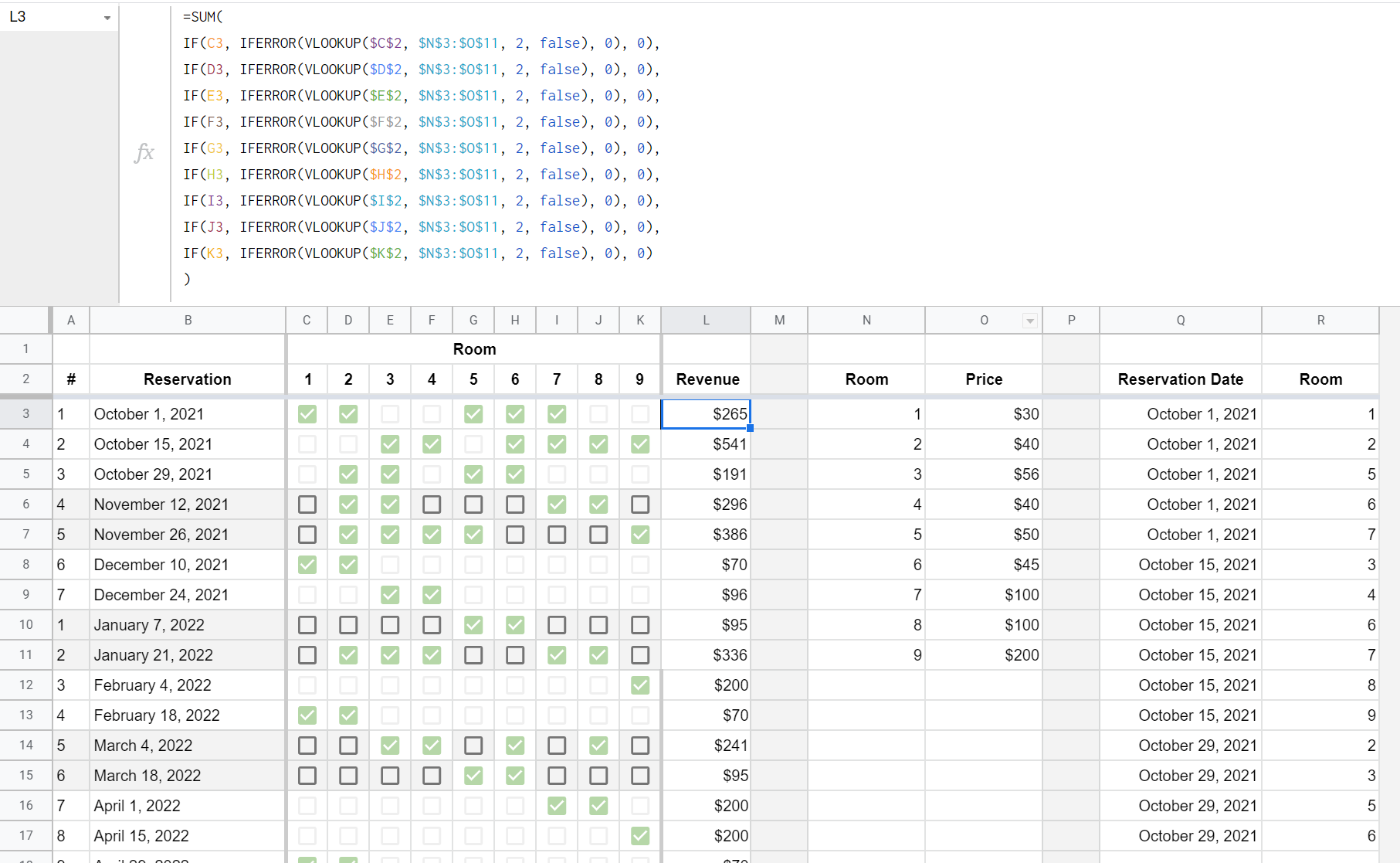
I have a situation where room reservations can be managed by checkboxes. You can see an example in the screenshot below. I've consolidated several sheets into one to provide visualization but the data lives in separate sheets in the actual document...

 1. Columns A-L are a "Manage Reservations" sheet.
 2. Columns N-O are a "Pricing" sheet.
 3. Columns Q-R would be the output on a "Reservation
    Calendar" sheet.

I have two questions:

1. Is there a better way to calculate revenue in column L?

The method I'm using is working but it's a beast to manage, doesn't feel efficient and I'm sure there's some swankier way to do a lookup and SUM of the checkboxes / room number -> room rate.

2. How can I output the data in columns B-K (that represents the reservations) into what is shown in column Q-R?

I can't seem to figure out a way to QUERY or PIVOT the checkboxes and dates they represent into individual rows in another sheet. I had first tried some PIVOT tables but was running into issues with, what I gather is the source data formatting.

I'd like to keep the formatting of columns A-L, if possible. It's easy to manage and visualize. That said, if it needs to change to optimize the calculations and allow for me to get the output of columns O-P on another sheet... I'll take that as a lesson in better spreadsheet architecting.

Sample Reference Data Sheet

Any help would be appreciated!

Answer 1

You want an efficient alternative to calculate revenue in column L.

Try this formula in the Cell L3 (based on the sample data below:

=arrayformula(sumproduct(C3:K3,pricing!$D$2:$L$2))

Sumproduct multiples, then sums, the values in multiple arrays. Note that the pricing data has been transposed so that the data is taken row-wise.

Unfortunately, SUMPRODUCT can't be used in with ARRAYFORMULA, so you have to copy the formula down as many rows as required.

---

You want an alternative formula for displaying the data in Columns Q-R.

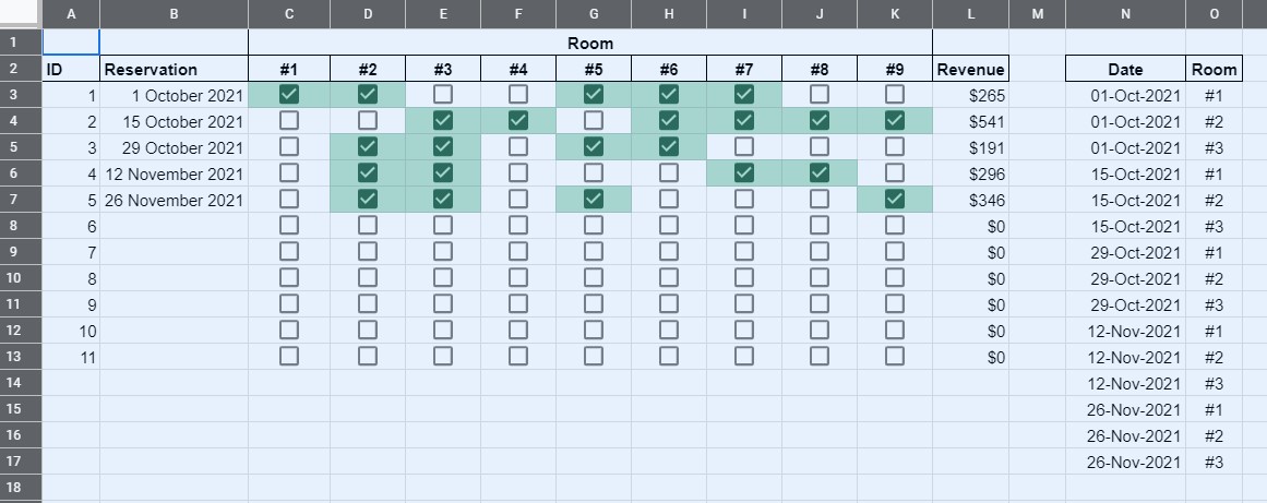
Try this formula: in cell N2 (based on the sample data below:

=query({"Date","Room","";ARRAYFORMULA({IFERROR(SPLIT(FLATTEN(IF(B3:B="",,B3:B&"♦"&C2:E2&"♦"&C3:E)), "♦"))})},"select Col1, Col2 format Col1 'dd-MMM-yyyy'")

This formula automatically populates the output for each row

---

Sample data and results

Answer 2

Since you're open to slight changes to your design, you can try this:

REVENUE:

=ARRAYFORMULA(IF(LEN(B4:B),MMULT(C2:K2*C4:K,TRANSPOSE(COLUMN(C2:K2)^0)), ))

SUMMARY BY DATES & ROOMS:

=ARRAYFORMULA(IF(LEN(B4:B),
sort(split(TO_DATE(B4:B)&"😊"&REGEXREPLACE(TRIM(
TRANSPOSE(QUERY(TRANSPOSE(
 IF((B4:K<>"")*(B4:K=TRUE), B3:K3&"-", )),,999^99))),
 "-$", )&"😊"&L4:L,"😊"),1,true),""))

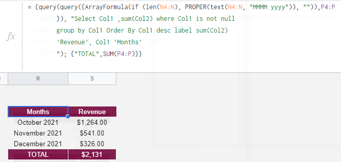
Summary by month:

For the fun you can also add this:

= {
    query(
        query({
            ArrayFormula(
                if (len(N4: N), PROPER(text(N4: N, "MMMM yyyy")), "")),
            P4: P
        }),
        "Select Col1 ,sum(Col2) where Col1 is not null 
        group by Col1 Order By Col1 desc label sum(Col2)
        'Revenue', Col1 'Months'
        "); {
            "TOTAL",
            SUM(P4: P)
        }
    }

SPREADSHEET DEMO: HERE