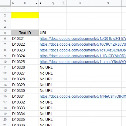
You need to use a couple of formula to resolve your question. There are many precedents for each element of those formula, but none that combine the specific combination of issues in your scenario.
1 - IMPORTRANGE - this will return a give range from an external spreadsheet. You include this formula in SheetB and import the URL/ID range from SheetA
2 - VLOOKUP - this formula goes in Sheet B, to lookup the ID in Column H in the imported range, and return the URL.
3 - VLOOKUP - range array- Vlookup searches in the first column of a range, but the first column of the imported range is the URL, so we use build an array (using curly brackets {}) to switch the two columns around.
4 - IFERROR - not every ID will have a URL. For those do not, use IFERROR to display an appropriate message.
5 - ARRAYFORMULA - you've got 300+ lines in sheet B, so use ARRAYFORMULA to automatically fill in all the rows from row#5 down to Row 300+
FORMULAS
Let's assume that you create a new sheet in Spreadsheet B called sheeta. And in Cell A2 of sheeta, you use this formula
=importrange("https://docs.google.com/spreadsheets/d/1q6AVzkK0NBCebqz2foJ-Uuj6ovAV1HG7AjRUyw2Qp-o/edit#gid=626967951","Sheet1!A2:B7")
- Step#2
In SpreadsheetB, Tab Y, use this formula in cell Q6
=ARRAYFORMULA(iferror(VLOOKUP(H6:H322,{sheeta!$B$2:$B$7,sheeta!$A$2:$A$7},2,FALSE),"No URL"))
IMPORTRANGE

LOOKUP URL


