Can I sum based on a specific cell text value?

Question

I have a spreadsheet for tracking sales leads. Each row is a lead. One of the columns is called "Status" and the options under this column are limited to a list of 4 options, i.e. Prospect, Proposal, Closed and Dead.

Is there a way for me to easily calculate how many rows have a status of Prospect vs how many have a status of Proposal, etc? I'd like to be able to have a summary at the top of the spreadsheet that shows how many of the leads are in each Status category (i.e. how many prospects vs proposals, etc).

Answer 1

Looks like you want to:

1. Make sure your data is validated (ie the user must choose one of those four options from a list so the data is clean)
2. Use a simple COUNTIF() statement to calculate the sum of various inputs.

Let's assume your user inputs are in COLUMN A

At the top of the spreadsheet (or anyplace you want to place your summary) you can write something like:

Column B    |  Column C
------------------------
Prospect    |  =countif(A:A,"Prospect")
Lead        |  =countif(A:A,"Lead")

Obviously to be more efficient, I would use cell references instead of the actual text (eg "Prospect," "Lead," etc) to define your criteria.

Example of using a cell reference rather than text: =countif(A:A,B2)

Answer 2

A pivot table may suit your expressed requirement - and possibly many others also:

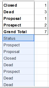
Add a column label to your data, if not already present, select it and your data, Data > Pivot table report..., Add field to Rows and Add field to Values. Ensure that the Values field is Summarise by: COUNTA (there is a little down arrow to click if necessary).

Copy the pivot table into the sheet above your data: