2

Is there a way to use the text value of cells with a conditional statement such as SUMIFS so that on one sheet I can have all the expenses:

#   A           B          C
1   R. Tusk     Travel     1,717.09
2   Frank U     Travel       634.67
3   R. Tusk     Meal          50.00
4   Frank U     Supplies   1,336.66
5   R. Tusk     Meal          10.00
6   R. Tusk     Meal          55.00
7   R. Tusk     Ent       23,803.97
8   R. Tusk     Pol. Don. 24,483.91
9   R. Tusk     Meal          10.03
10  R. Tusk     Ent        1,191.62
11  Frank U     Pol. Don. 40,493.14
12  R. Tusk     Pol. Don. 10,014.01
13  Frank U     Travel       100.00

and on the other sheet I can have essentially one formula the following?:

Politician      Meal        Travel    Pol. Don.        Ent     Supplies
R. Tusk         XXXX.XX    XXXX.XX      XXXX.XX    XXXX.XX      XXXX.XX
Frank U         XXXX.XX    XXXX.XX      XXXX.XX    XXXX.XX      XXXX.XX  

I was thinking:

=SUMIFS('Sheet1'!C:C,'Sheet1'!B:B,"=T(B$1)",'Sheet1'!A:A),"=T($A2)")

but that and other slight variations only gave me error, #N/A, and #Value!

Update For those playing at home, this worked:

=SUM(FILTER('Sheet1'!$C:$C,'Sheet1'!$B:$B=B$1,'Sheet1'!$A:$A=$A2))
0

2 Answers 2

1

With the following formula you can accomplish that.

Formula

=QUERY(DATA!D2:F15, "SELECT D, SUM(F) GROUP BY D PIVOT E LABEL D 'Politicians'")

Explained

The QUERY function will group the summation of the costs per politician and pivot the outcome per type.

Screenshot

enter image description here

Example

I've prepared an example for you: overview with query and pivot

1
  • The formula provided by Jacob Jan Tuinstra is awesome. You could also use Pivot Table: trendct.org/2015/09/04/…. Surprisingly easy to do.
    – Paola
    Commented Oct 31, 2017 at 17:25
0

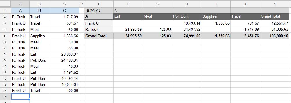
By a fairly narrow margin I would prefer a pivot table for this (as suggested by @Paola). These are a good choice where different views of the same data may be required but in this case the decider for me is the ease (automatic) of adding totals by column and row. (The fancy new layout was an influence too!):

WA61061 example

Just select the data (and column headers), Data, Pivot table..., and select to suit.

The alphabetical sort is also automatic as is placement on a different sheet (I moved it for the sake of the image).

Your Answer

By clicking “Post Your Answer”, you agree to our terms of service and acknowledge you have read our privacy policy.

Not the answer you're looking for? Browse other questions tagged or ask your own question.