Corrected spelling, improved formatting, inlined screenshot
Source Link
Alex
  • 22.8k
  • 12
  • 83
  • 104

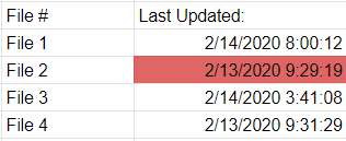
I have a Google sheet that has a column for "last updated" and each row represents a separate file. People manually paste in the time and date in that column, like in the screenshot.

If the date and time is not within the last 24 hours, then I want that cell to turn red. The "date is before" option only checks the date and not the time.

For this example, let's say the current time is 930 AM, so the cells that have a time before 9:30 AM yesterday should turn red. The cells that have a time after 9:30 AM yesterday should remain unaffected.

This is what I want it to look like.

This is what I want it to look like

How can I do this with Google Sheets conditional formatting?

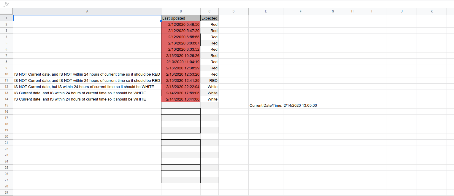
Here is my test sheet.

enter image description here
(Click image to enlarge)

https://docs.google.com/spreadsheets/d/1DRQYrxpE61e7VMEpbuiCO543cpZvcckVr0PKPnQcPw4/edit?usp=sharing

I have a Google sheet that has a column for "last updated" and each row represents a separate file. People manually paste in the time and date in that column, like in the screenshot.

If the date and time is not within the last 24 hours, then I want that cell to turn red. The "date is before" option only checks the date and not the time.

For this example, let's say the current time is 930 AM, so the cells that have a time before 9:30 AM yesterday should turn red. The cells that have a time after 9:30 AM yesterday should remain unaffected.

This is what I want it to look like.

This is what I want it to look like

How can I do this with Google Sheets conditional formatting?

Here is my test sheet.

enter image description here
(Click image to enlarge)

https://docs.google.com/spreadsheets/d/1DRQYrxpE61e7VMEpbuiCO543cpZvcckVr0PKPnQcPw4/edit?usp=sharing
Corrected spelling, improved formatting, inlined screenshot
Source Link

Conditional formatting for cells that have date/time withingwithin the last 24 hours

Ok so I have a Google sheet that has a colcolumn for "last updated" and each row represents a separate file. People manually paste in the time and date in that colcolumn, just like in the picturescreenshot.

If the date and time IS NOTis not within the last 24 hours, then I want that cell to turn red. The "date is before" option only checks the date and not the time.

For this example, let's say the current time is 930am930 AM, so the cells that have a time BEFOREbefore 9:30am30 AM yesterday should turn red. The cells that have a time AFTERafter 9:30am30 AM yesterday should remain unaffected.

This is what I want it to look like This is what I want it to look like.

This is what I want it to look like

How can I do this with Google Sheets conditional formatting? How can I do this with Google Sheets conditional formatting?

Here is my Testtest sheet:.

enter image description here
https://docs.google.com/spreadsheets/d/1DRQYrxpE61e7VMEpbuiCO543cpZvcckVr0PKPnQcPw4/edit?usp=sharing(Click image to enlarge)

Conditional formatting for cells that have date/time withing the last 24 hours

Ok so I have a Google sheet that has a col for "last updated" and each row represents a separate file. People manually paste in the time and date in that col, just like in the picture.

If the date and time IS NOT within the last 24 hours, then I want that cell to turn red. The "date is before" option only checks the date and not the time.

For this example, let's say the current time is 930am, so the cells that have a time BEFORE 9:30am yesterday should turn red. The cells that have a time AFTER 9:30am yesterday should remain unaffected.

This is what I want it to look like

This is what I want it to look like

How can I do this with Google Sheets conditional formatting?

Here is my Test sheet: https://docs.google.com/spreadsheets/d/1DRQYrxpE61e7VMEpbuiCO543cpZvcckVr0PKPnQcPw4/edit?usp=sharing

Conditional formatting for cells that have date/time within the last 24 hours

I have a Google sheet that has a column for "last updated" and each row represents a separate file. People manually paste in the time and date in that column, like in the screenshot.

If the date and time is not within the last 24 hours, then I want that cell to turn red. The "date is before" option only checks the date and not the time.

For this example, let's say the current time is 930 AM, so the cells that have a time before 9:30 AM yesterday should turn red. The cells that have a time after 9:30 AM yesterday should remain unaffected.

This is what I want it to look like.

This is what I want it to look like

How can I do this with Google Sheets conditional formatting?

Here is my test sheet.

enter image description here
(Click image to enlarge)

Became Hot Network Question
added 67 characters in body
Source Link

Ok so I have a Google sheet that has a col for "last updated" and each row represents a separate file. People manually paste in the time and date in that col, just like in the picture.

If the date and time IS NOT within the last 24 hours, then I want that cell to turn red. The "date is before" option only checks the date and not the time.

For this example, let's say the current time is 930am, so the cells that have a time BEFORE 9:30am yesterday should turn red. The cells that have a time AFTER 9:30am yesterday should remain unaffected.

This is what I want it to look like

This is what I want it to look like

How can I do this with Google Sheets conditional formatting?

Here is my Test sheet: https://docs.google.com/spreadsheets/d/1DRQYrxpE61e7VMEpbuiCO543cpZvcckVr0PKPnQcPw4/edit?usp=sharing

Ok so I have a Google sheet that has a col for "last updated" and each row represents a separate file. People manually paste in the time and date in that col, just like in the picture.

If the date and time IS NOT within the last 24 hours, then I want that cell to turn red.

For this example, let's say the current time is 930am, so the cells that have a time BEFORE 9:30am yesterday should turn red. The cells that have a time AFTER 9:30am yesterday should remain unaffected.

This is what I want it to look like

This is what I want it to look like

How can I do this with Google Sheets conditional formatting?

Here is my Test sheet: https://docs.google.com/spreadsheets/d/1DRQYrxpE61e7VMEpbuiCO543cpZvcckVr0PKPnQcPw4/edit?usp=sharing

Ok so I have a Google sheet that has a col for "last updated" and each row represents a separate file. People manually paste in the time and date in that col, just like in the picture.

If the date and time IS NOT within the last 24 hours, then I want that cell to turn red. The "date is before" option only checks the date and not the time.

For this example, let's say the current time is 930am, so the cells that have a time BEFORE 9:30am yesterday should turn red. The cells that have a time AFTER 9:30am yesterday should remain unaffected.

This is what I want it to look like

This is what I want it to look like

How can I do this with Google Sheets conditional formatting?

Here is my Test sheet: https://docs.google.com/spreadsheets/d/1DRQYrxpE61e7VMEpbuiCO543cpZvcckVr0PKPnQcPw4/edit?usp=sharing

added 123 characters in body
Source Link
Loading
added 1 character in body
Source Link
marikamitsos
  • 13.1k
  • 4
  • 34
  • 59
Loading
added 13 characters in body
Source Link
Loading
Source Link
Loading