edited body
Source Link
marikamitsos
  • 13.1k
  • 4
  • 34
  • 59

You can try the following formula

=ArrayFormula((V3V2:V6&"V5&"-"&MONTH(T3T2:T6T5)&"-"&DAY(T3T2:T6T5))*1)

enter image description here

(Please adjust ranges to your needs)

If you want to apply for the whole range you can use:

=ArrayFormula(IF(V2:V="",,(V2:V&"-"&MONTH(T2:T)&"-"&DAY(T2:T)*1)))  

EDIT

Following OP's request

I actually wanted to keep this in the Datevalue format, e.g. 44116 instead of 10/12/2020.

Please use the following arrayformula

=ArrayFormula(IF(V2:V="",,((V2:V&"-"&MONTH(T2:T)&"-"&DAY(T2:T))*1)))

DO notice the extra parenthesis. They make all the difference.
Using this second formula you get the results as datevalues. If you then want to have them as dates, you can format them from the Format -->Number -->Date menu according to your preferences.

Functions used:

You can try the following formula

=ArrayFormula((V3:V6&"-"&MONTH(T3:T6)&"-"&DAY(T3:T6))*1)

enter image description here

(Please adjust ranges to your needs)

If you want to apply for the whole range you can use:

=ArrayFormula(IF(V2:V="",,(V2:V&"-"&MONTH(T2:T)&"-"&DAY(T2:T)*1)))  

EDIT

Following OP's request

I actually wanted to keep this in the Datevalue format, e.g. 44116 instead of 10/12/2020.

Please use the following arrayformula

=ArrayFormula(IF(V2:V="",,((V2:V&"-"&MONTH(T2:T)&"-"&DAY(T2:T))*1)))

DO notice the extra parenthesis. They make all the difference.
Using this second formula you get the results as datevalues. If you then want to have them as dates, you can format them from the Format -->Number -->Date menu according to your preferences.

Functions used:
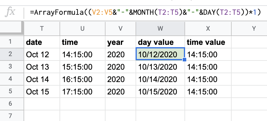
You can try the following formula

=ArrayFormula((V2:V5&"-"&MONTH(T2:T5)&"-"&DAY(T2:T5))*1)

enter image description here

(Please adjust ranges to your needs)

If you want to apply for the whole range you can use:

=ArrayFormula(IF(V2:V="",,(V2:V&"-"&MONTH(T2:T)&"-"&DAY(T2:T)*1)))  

EDIT

Following OP's request

I actually wanted to keep this in the Datevalue format, e.g. 44116 instead of 10/12/2020.

Please use the following arrayformula

=ArrayFormula(IF(V2:V="",,((V2:V&"-"&MONTH(T2:T)&"-"&DAY(T2:T))*1)))

DO notice the extra parenthesis. They make all the difference.
Using this second formula you get the results as datevalues. If you then want to have them as dates, you can format them from the Format -->Number -->Date menu according to your preferences.

Functions used:

added 449 characters in body
Source Link
marikamitsos
  • 13.1k
  • 4
  • 34
  • 59

You can try the following formula

=ArrayFormula((V3:V6&"-"&MONTH(T3:T6)&"-"&DAY(T3:T6))*1)

enter image description here

(Please adjust ranges to your needs)

If you want to apply for the whole range you can use:

=ArrayFormula(IF(V2:V="",,(V2:V&"-"&MONTH(T2:T)&"-"&DAY(T2:T)*1)))  

EDIT

Following OP's request

I actually wanted to keep this in the Datevalue format, e.g. 44116 instead of 10/12/2020.

Please use the following arrayformula

=ArrayFormula(IF(V2:V="",,((V2:V&"-"&MONTH(T2:T)&"-"&DAY(T2:T))*1)))

DO notice the extra parenthesis. They make all the difference.
Using this second formula you get the results as datevalues. If you then want to have them as dates, you can format them from the Format -->Number -->Date menu according to your preferences.

Functions used:

You can try the following formula

=ArrayFormula((V3:V6&"-"&MONTH(T3:T6)&"-"&DAY(T3:T6))*1)

enter image description here

(Please adjust ranges to your needs)

If you want to apply for the whole range you can use:

=ArrayFormula(IF(V2:V="",,(V2:V&"-"&MONTH(T2:T)&"-"&DAY(T2:T)*1)))

Functions used:

You can try the following formula

=ArrayFormula((V3:V6&"-"&MONTH(T3:T6)&"-"&DAY(T3:T6))*1)

enter image description here

(Please adjust ranges to your needs)

If you want to apply for the whole range you can use:

=ArrayFormula(IF(V2:V="",,(V2:V&"-"&MONTH(T2:T)&"-"&DAY(T2:T)*1)))  

EDIT

Following OP's request

I actually wanted to keep this in the Datevalue format, e.g. 44116 instead of 10/12/2020.

Please use the following arrayformula

=ArrayFormula(IF(V2:V="",,((V2:V&"-"&MONTH(T2:T)&"-"&DAY(T2:T))*1)))

DO notice the extra parenthesis. They make all the difference.
Using this second formula you get the results as datevalues. If you then want to have them as dates, you can format them from the Format -->Number -->Date menu according to your preferences.

Functions used:

deleted 5 characters in body
Source Link
marikamitsos
  • 13.1k
  • 4
  • 34
  • 59

You can try the following formula

=ArrayFormula((V3:V6&"-"&MONTH(T3:T6)&"-"&DAY(T3:T6))*1)

enter image description here

(Please adjust ranges to your needs)

If you want to apply for the whole range you can use:

=ArrayFormula(IF(V2:V="",,(V2:V&"-"&MONTH(T2:T)&"-"&DAY(T2:T)*1)))

Functions used:

You can try the following formula

=ArrayFormula((V3:V6&"-"&MONTH(T3:T6)&"-"&DAY(T3:T6))*1)

enter image description here

(Please adjust ranges to your needs)

If you want to apply for the whole range you can use:

=ArrayFormula(IF(V2:V="",,(V2:V&"-"&MONTH(T2:T)&"-"&DAY(T2:T)*1)))

Functions used:

You can try the following formula

=ArrayFormula((V3:V6&"-"&MONTH(T3:T6)&"-"&DAY(T3:T6))*1)

enter image description here

(Please adjust ranges to your needs)

If you want to apply for the whole range you can use:

=ArrayFormula(IF(V2:V="",,(V2:V&"-"&MONTH(T2:T)&"-"&DAY(T2:T)*1)))

Functions used:

Source Link
marikamitsos
  • 13.1k
  • 4
  • 34
  • 59
Loading