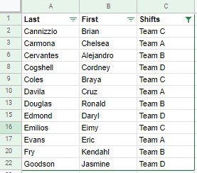
You want to "filter" a list of names (with shift groups) based on shift groups.
Option#1 - Filter (menu)
=arrayformula(ifna(match(C2:C22,Shifts!$B$2:$B$5,0),0))>0
Filterthe "Shifts" column- select
Filter by Condition - select
Custom formula - enter the formula.
- select
Using match, the formula returns the index value of a match between Shifts (Column C2:C22) and the values in the "Tuesday" column of the "Shifts" sheet (Shifts!$B$2:$B$5). If there is no match, the formula returns a value of zero. By making the condition = >0, the formula will return only those matching values.
This formula has a disadvantage - the filtered day from the Shifts sheet is hard-coded which makes it inconvenient to change.
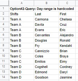
Option#2 - Query: hardcoded 'day'
=query(Names!A1:C22,"select C, A, B where "&"C='"&textjoin("' OR C = '",true,Shifts!B2:B5)&"' order by C",1)
Enter this formula in any sheet, and it will return the same information as the filter option.
- Note, that filtered day from the
Shiftssheet is hard-coded.
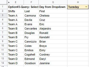
Option#3-Query: Select Day from Dropdown
=query(Names!A1:C22,"select C, A, B where "&"C='"&textjoin("' OR C = '",true,indirect(address(2,match($H$1,Shifts!A1:G1,0),4,true,"Shifts")&":"&address(100,match($H$1,Shifts!A1:G1,0),4)))&"' order by C",1)
- Enter the formula in any cell
- Create a Data Validation dropdown (cell H1) by referencing the range
=Shifts!$A$1:$G$1.
The formula now references the "day" by matching the dropdown value. This approach makes it easy to modify data reporting.


