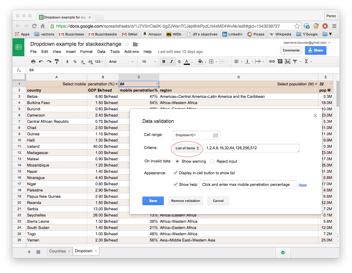
See thethis example spreadsheet. Sheet Countries contains source data (instead of prices and products, I've used countries, population and other data, but the concept is the same). Sheet Dropdown contains the example. In that latter sheet, cell C1 and E1 are dropdown menus (use the Data→Validation… menu to see how data validation works, or look at the explanations at the bottom of this answer).
Then, in cell A2, you have a query that fetches data from the Countries sheet, based on the values present in your dropdown menus. The trick is to build the query string using the string concatenation operator (&). What the query string says is: fetch data from columns A to E of the Countries sheet, where column C is lower than Dropdown!C1 and column E is lower than Dropdown!E1.
Note that you will need to copy the example spreadsheet to play with it (you can only comment the original).
Explanations
To set a cell as a drop down menu, select the cell, then use the Data→Validation… menu. For instance, for cell C1 of the Dropdown sheet, you can enter the list of values you want users to select from by setting the
 Criteria to List of items and then enter comma separated values in the input box right next to it. Other options of this validation menu are self explanatory.
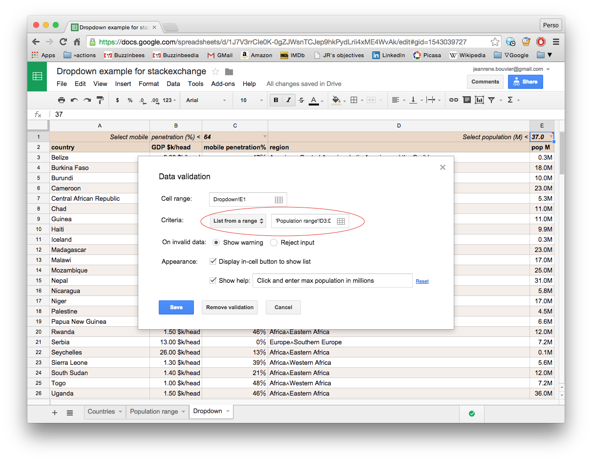
Another common dropdown menu is where you want users to select values from a range within the spreadsheet:  As you can see here, the
 Criteria is now set to List from a range. You enter the range itself by clicking on the grid within the input box, and then by selecting the range of cells you want to use as your selectable items. In the case of our examples, the values come from the sheet Population range where I made some computations to generate a log scale list of values between the smallest country population and the largest.
Hope this helps.
