If certain dropdown, counting another number on the same row

Question

This is pretty basic I'm assuming, but I'm rather inexperienced.

So I have a dropdown list of categories. On every row I also have a column of numbers. I want to have totals of each category's number.

Example:

• Dog 2
• Cat 1
• Duck 3
• Dog 4
• Cat 6

Total Dog: 6
Total Cat: 7
Total Duck: 3

Answer 1

I would use query for this. Assuming your data is in columns A:B, the query would look like

=query(A:B, "select A, sum(B) group by A")

Answer 2

Assuming you data sample is just a sample, I would favour a pivot table:

Animal to Add field Rows and No. to Add field Values.

Answer 3

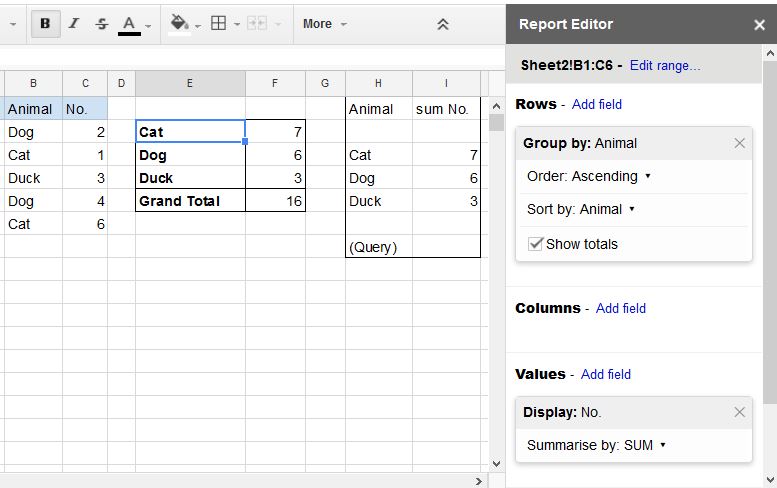
For your example, I think SUMIF is a good option.

The syntax is SUMIF(range, criterion, [sum_range])

See https://support.google.com/docs/answer/3093583?hl=en for more info.

For example,

|   |   A  | B | C |   D    |           E              |
|---|------|---|---|--------|--------------------------|
| 1 | Dog  | 2 |   | Totals |                          |
| 2 | Cat  | 1 |   | Dog    | =SUMIF(A1:A5, D2, B1:B5) |
| 3 | Duck | 3 |   | Cat    | =SUMIF(A1:A5, D3, B1:B5) |
| 4 | Dog  | 4 |   | Duck   | =SUMIF(A1:A5, D4, B1:B5) |
| 5 | Cat  | 6 |   |        |                          |

Columns D and E have the sum totals of columns A and B.

The first value is A1:A5 because those cells have the column we are testing.

The second value is either D2, D3, or D4, depending on what we are testing against.

The third value is B1:B5 because that have the values we want to sum.