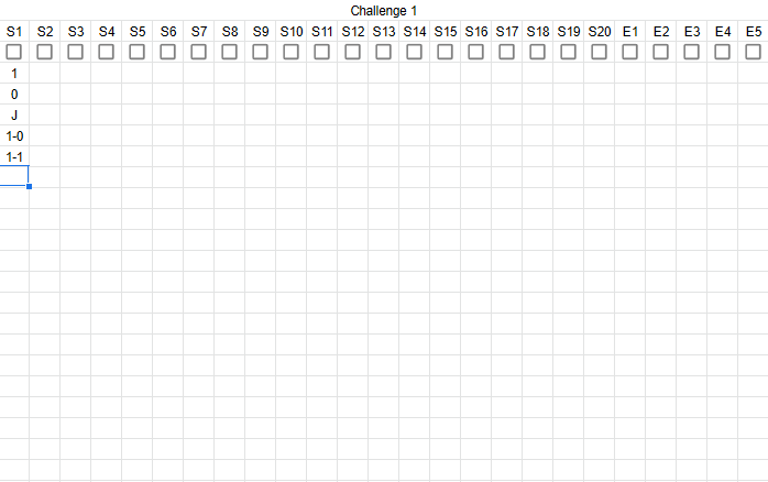
So I'm making this attendance tracker for my school, and I need to apply a different format depending on the value of the cell and if a checkbox is ticked or not. Here is a screenshot of the different values to be applied and the checkboxes

The different values dictate:

• 1= 1 hour class, student attended
• 0= 1/2 hour class, student didn't attend
• J= Student has a justified absence
• 1-0= 2 hour class, student only attended for 1 hour
• 1-1= 2 hour class, student attended both hours

It is important for the values to represent if it's a 2 hour or a 1 hour class, so maybe using an operator is not the best choice but it was the one that ocurred to me. (If you happen to have a better arrangement I'm all ears)

So the main point is: I need each of the cells to check the Checkbox for the column to verify if that class has been given by the teacher, and then check the vaule inside of the cell to change its format and apply a color to the cell.(eg. Green for attendance, red for absence, blue for justified, etc)

And another point is that I have to make another formula that chacks how many boxes are ticked and give me a number of classes given, so I can get a percentage of classes attended depending on the classes given.

I've been struggling with this for a while and apologies if the explanation is long as heck.

EDIT: Here is an example document with the desired results. Example document