Good day, everyone! ^^
I am still a beginner in Google Sheets formulas and still don't understand many things, but I am trying to scrape sample sentences from an online Japanese dictionary using IMPORTXML in a spreadsheet.
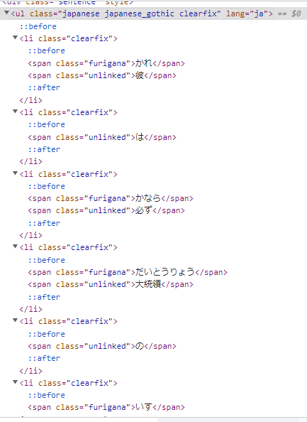
As shown on the image above, some ul descendants are categorized by 2 different span @classes, or has sibling, from some li parents.
<span class="furigana"> ***
<span class="unlinked">
***[for those who don't know] [for those who don't know] furigana, in Japanese, is basically their assigned phonetic character as reading aid for their Kanji letters (characters borrowed or adapted from Chinese writing)furigana, in Japanese, is basically their assigned phonetic character as reading aid for their Kanji letters (characters borrowed or adapted from Chinese writing)*
And on the other hand, other li parents has 1 child only, and that is
<span class="unlinked">
My goal is to split @class='furigana' and @class='unlinked' into 2 separate columns and those 'unlinked' characters that doesn't have any 'furigana' counterpart will be replaced with — symbol instead of a blank cell.
I haven't done any filtering on my formula yet, but here it is:
= IMPORTXML( "https://jisho.org/word/%E6%A4%85%E5%AD%90", "//span[@class='furigana']/ancestor::ul[@class='japanese japanese_gothic clearfix']/li[@class='clearfix']" )
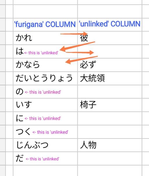
What happened was my formula miraculously gave me 2 columns for some reason that I don't understand, which is somewhat beneficial on my part, and seemingly already separated some 'unlinked' characters from the 'furigana' column. But I think it only segregated the characters in zigzag order, that's why some 'unlinked' characters are on the 'furigana' side.
I hope someone could help me and provide some simple formula that I could easily comprehend. My English is not that good as well so please bear with me. And from the bottom of my heart, THANK YOU SO MUCH in advance! Y_Y
Have a blessed day, everyone!


