3

I have a column of phone numbers in that are in different formats. I want them all to be in this format 0000 000 000.

What I do now is manually edit each wrong number into the correct format.

How can I use a filter or conditional formatting to find all numbers that are NOT in this format (#### ### ###).

Here is the sample sheet:
https://docs.google.com/spreadsheets/d/1rlATwRPTkofEg0rB5-GSwwBpQDa7ZOoeNvhs0xPOsKA/edit?usp=sharing

2
  • Please manually enter into Column D what you expect the result to be for EACH of the 9 samples you've listed in Column A. As it stands, there is not enough information to go on with just one conversion shown, since some of your listings have just 8 digits, some have 9, some have 10 (the target number), and some have more than 10. If you add or remove digits to get the manual format, explain in Column E how you determined where those digits should be added or which should be deleted.
    – Erik Tyler
    Commented Jan 5, 2021 at 8:10
  • That's actually the thing. Sometimes the numbers show up in the incorrect format, that is how the customers have entered it. I want to spot just those that are in the wrong format.
    – Genny
    Commented Jan 5, 2021 at 10:40

3 Answers 3

2

Addressing strictly what you've requested in your post, I added a sheet ("Erik Help") with a custom conditional formatting rule applied to Column A:

=AND(LEN(A1),ISERROR(REGEXEXTRACT(A1,"^\d{4}\s\d{3}\s\d{3}$")))

This will highlight any entries in Column A that are not in the format "#### ### ###".

You can view this rule by clicking any cell in Column A, then choosing from the menu Format > Conditional formatting and double clicking on the rule that appears.

Two conditions must me met for the rule to take effect:

  1. LEN(A1) means the cell must have something in it (i.e., it has LENgth).
  2. The contents of the cell produce an (IF)ERROR when trying to (REGEX)MATCH the regular expression.

The regular expression means "startofstring-digits(four)-space-digits(3)-space-digits(3)-endofstrong."

2
  • Thank you so much. It works like magic. And thank you for the explanation too! :D (I'm actually on the fence about whether I should mark you or marikmitsos as the correct answer because both work)
    – Genny
    Commented Jan 6, 2021 at 2:33
  • 1
    We don't win any prizes for "Best Answer." We're all volunteers. The main thing is to mark someone's answer as "Best Answer," so that contributors can see at a glance from the main issues page which issues have been resolved. So thank you for doing that.
    – Erik Tyler
    Commented Jan 6, 2021 at 4:09
3

You mentioned

How can I use a filter or conditional formatting to find all numbers that are NOT in this format (#### ### ###).

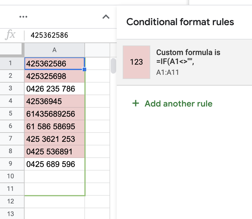
Please use the following conditional-formatting rule

=IF(A1<>"",(IF(ISNUMBER(A1),TRUE,NOT(REGEXMATCH(A1,"^\d{4} \d{3} \d{3}$")))))

enter image description here

4
  • 1
    you and I had similar thinking; however, your rule would fail to flag entries like "10425 689 5967" that contain the desired pattern without being limited to only that pattern because you don't have the startofstring and endofstring markers. I'd recommend adding those.
    – Erik Tyler
    Commented Jan 5, 2021 at 16:09
  • Seasons greetings @ErikTyler You were right. I had written a testing formula instead of my final one. It is now fixed. Commented Jan 5, 2021 at 16:33
  • 1
    Hey @marikamitsos Thank you so much again for your help! It works like magic! I'm on the fence about whether to mark you or Erik as the correct answer, because both your formulas work.
    – Genny
    Commented Jan 6, 2021 at 2:34
  • 1
    Seasons greetings @Genny No worries. The only difference is that my formula takes into account the fact that data column can also have letters down the line while Erick's formula does not. Commented Jan 6, 2021 at 9:43
2
  1. First substitute the white space. Paste this to Cell B2: =SUBSTITUTE(A2, " ", "")
  2. After that make your number to exactly 10 digit. Paste this to Cell C2:
    =IF(LEN(B2)=9,"0"&B2, IF(LEN(B2)=8,"00"&B2, IF(LEN(B2)=10,B2)))
  3. Lastly add the space back to the right place.Paste this to Cell D2:
    =LEFT(C2,4)&" "&MID(C2,4,3) &" " &right(C2,3)

you shall have your expected result already. just that ur sample there, having cell with 12 digit, I don't know what kind of expected result for that.

1
  • Hi Xylan, thank you for your answer. It is useful, but my issue is this is in one column and I want to be able to find a solution without having to add other columns. I've edited my original question now a bit, sorry.
    – Genny
    Commented Jan 5, 2021 at 10:41

Your Answer

By clicking “Post Your Answer”, you agree to our terms of service and acknowledge you have read our privacy policy.

Not the answer you're looking for? Browse other questions tagged or ask your own question.