0

I hope someone could help with this one. I’m not sure if this is possible but I would like to know if there is any way to insert a blank row after every change of Data in ColumnA(Country) which is the result of a query function.

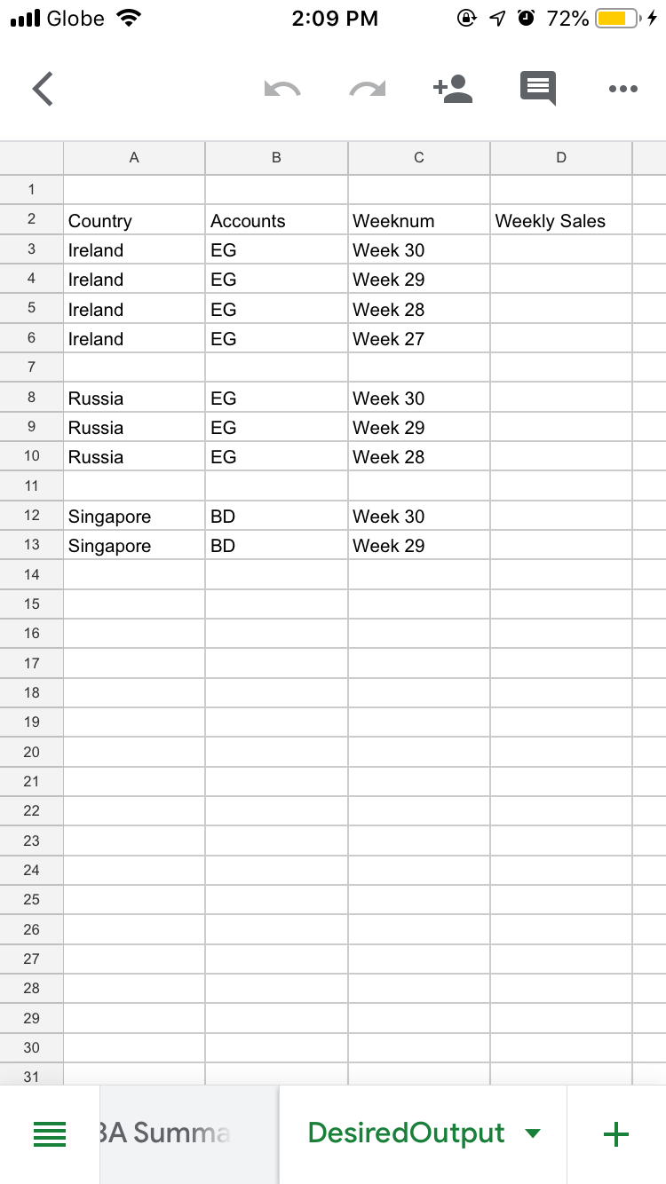
I want to break on Country (Column A) and Accounts" (Column B) as per the DesiredOutput sheet.

Here is the sample file:

https://docs.google.com/spreadsheets/d/10R3pOblC3_u6E5-l1LqvaZzMlrZWoVuYrebVMW2wm9w/edit

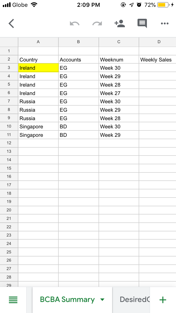
BCBA Summary tab is the result of the query referencing the Raw_Data tab. enter image description here
The DesiredOutput tab is my aim since I will have more than 20 accounts that will be added in the future and it will be easier for me to read the data.

enter image description here

I wonder if there is any way to get the DesiredOutput?

I tried this How to automatically insert a blank row after a group of data, successfully inserted a row, however, it is for every other data. I hope you could help me.

Thank you so much.

4
  • Welcome. Would you please add a brief description of your search/research efforts..
    – Tedinoz
    Commented Aug 9, 2020 at 12:50
  • You need whole row blank, totals per country from Pivot table won't do?
    – Oleg_S
    Commented Aug 13, 2020 at 7:33
  • @Oleg S that could be possible with a Pivot table, yes, however, I am trying to make the sheet formula based to make it more dynamic and to avoid manually adjusting the range every time there are new data.
    – Xan Mei
    Commented Aug 13, 2020 at 20:17
  • @XanMei Would you please update your question to show that you want to break on Country (Column A) and Accounts" (Column B) as per the "Desired Output" sheet in your spreadsheet.
    – Tedinoz
    Commented Aug 14, 2020 at 2:53

1 Answer 1

1

You want to insert a new line at each change of Country (Column A).

There are many ways that this could be done. These have been sourced from: How to automatically insert a blank row after a group of data. on Google Docs Help (Community).

Option #1, based on TEXTJOIN():

=ArrayFormula(iferror(split(transpose(split(textjoin(",",true,if(len('BCBA Summary'!A3:A),{'BCBA Summary'!A3:D,if('BCBA Summary'!A3:A<>'BCBA Summary'!A4:A,";;",";")},)),";",true,false)),",",true,true)))

OR

Option #2, based on VLOOKUP(), SORT() and FILTER():

=ARRAYFORMULA(IFERROR(VLOOKUP(SORT({FILTER(ROW('BCBA Summary'!A3:A),'BCBA Summary'!A3:A<>"");FILTER(ROW('BCBA Summary'!A3:A),'BCBA Summary'!A3:A<>"",'BCBA Summary'!A3:A<>'BCBA Summary'!A4:A)+0.5}),{ROW('BCBA Summary'!A3:A),'BCBA Summary'!A3:D},{2,3,4,5},0)))

Both formula yield the same result.

2
  • Thank you for this one @Tedinoz. I will certainly try this on Monday.
    – Xan Mei
    Commented Aug 14, 2020 at 22:05
  • Thank you for your answer @Tedinoz. It is working properly. You really help me a lot. This is the answer I am looking for. I really appreciate your help. :-)
    – Xan Mei
    Commented Aug 17, 2020 at 16:05

Your Answer

By clicking “Post Your Answer”, you agree to our terms of service and acknowledge you have read our privacy policy.

Not the answer you're looking for? Browse other questions tagged or ask your own question.