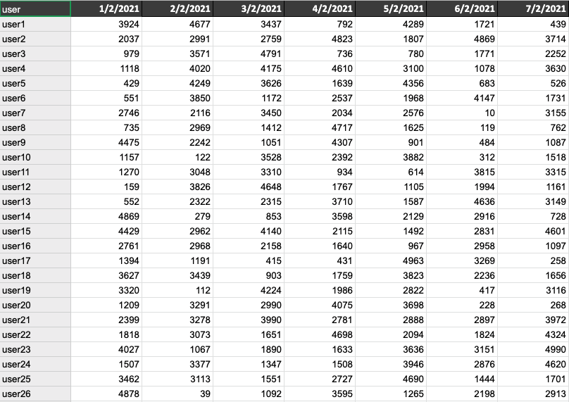
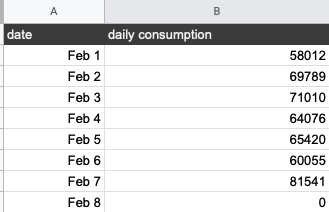
My solution does not refer to your existing sheets at all. I've added two sheets ("Master" and "Erik Help") to your sample spreadsheet, both tabs highlighted with bright green. The "Master" sheet is hidden (which I would recommend, because you won't need it in daily dealings. You can see it and Unhide it if you like by clicking the icon of three stacked bars at the bottom left of the spreadsheet.
When any more than one cell of data will be used in conjunction with IMPORTRANGE, I nearly always recommend importing the entire data set from the external sheet to its own sheet in the processing spreadsheet, then referring to that full data sheet (rather than IMPORTRANGE formulas) for anything you need to do in the processing spreadsheet.
Note the structure of the IMPORTRANGE formula in Master!A1:
=IMPORTRANGE("1JwbcOmfoRgc4s4OVN4poQ18KLWbqY2tZ22NA07ZsZIg","Sheet1!A1:"&ROWS(IMPORTRANGE("1JwbcOmfoRgc4s4OVN4poQ18KLWbqY2tZ22NA07ZsZIg","Sheet1!A:A")))
This is flexible, in that it brings in "everything," even if you add rows or columns to the external sheet.
Then, in the "Erik Help" sheet, I refer to that hidden Master sheet only, since it now contains all the data I need.
The formula in "Erik Help," cell A1, is similarly written to be flexible — contracting or expanding as the Master data set contracts or expands. For instance, as you continue to add more days' data to the external sheet, both of my formulas will "keep up" with that, without the need to adjust them in order to continue getting updated results. Here is the 'Erik Help'!A1 formula:
=ArrayFormula(TRANSPOSE({FILTER(Master!B1:1,Master!B1:1<>"");MMULT(SEQUENCE(1,ROWS(Master!A2:A),1,0),FILTER(IF(ISNUMBER(INDIRECT("Master!B2:"&ROWS(Master!A:A))),INDIRECT("Master!B2:"&ROWS(Master!A:A)),0),Master!B1:1<>""))}))
This will produce a TRANSPOSEd version of the following array:
A FILTERed array consisting of any cells in Master!B1:1 that are not blank (i.e., that contain dates). This allows that range to expand and contract.
An MMULT ("Matrix Multiplication") calculation of a FILTERed array of all the numbers from B2 over where B1:1 is not blank.
I recommend you study MMULT; while difficult for many to wrap their head around initially, it's quite powerful. My short notes:
Every element in the MMULT grid must be a number (which is why you see my formula checks ISNUMBER and assigns a value of 0 to anything that isn't already a number.
MMULT multiplies one matrix (i.e., grid) by another. That is, it multiplies every value per row of the first matrix by every value per column of the second and then adds up all these values. (If you think about it, that's exactly what you are trying to do by "adding up every separate column of values.")
Therefore, the number of columns in the first matrix must be equal to the number of rows in the second matrix (or vice versa). By setting one of those matrices to a long column or row consisting only of repeated 1's, you are actually adding, because anything multiplied by 1 is itself.
Here is a graphic I prepared that might better explain MMULT and what it does:

I do want to point out that your dates are perhaps not representing what you think they do currently. It seems to me that you think your dates are currently representing the dates of the first week of February. In fact, they are representing the second day of each month from January to July. That is, your date format (perhaps for your region) is showing d/m/yyyy format rather than m/d/yyyy. That is something you'll need to correct at the source (by writing your dates in m/d/yyy format). Otherwise, you'll begin to see real problems as soon as February 13 is added, because 13 cannot be translated to a month, and so the values from there to the end of each month will show as a string instead of a real date.


