Return every column header that contains a value

Question

I'm trying to return the header of every column in which a value appears, and put these headers in one cell separated by commas e.g. if "xyz" is contained within columns titled Column1 and Column7, then this formula would return "Column1, Column7" in the cell.

• The headers of the column are in Row H4:AF4

• The data is underneath, in H5:AF99

• The value I'm looking up sits in cell E1

At the moment this formula is working for some values, but not all:

=JOIN(", ",QUERY(TRANSPOSE(H4:AL99),"Select Col1 where "&JOIN(" or ",ARRAYFORMULA("Col"&(COLUMN(H4:AL4)-COLUMN(H4)+1)&" = '"&$E$1&"'"))))

Can anyone explain why this formula works for some of my lookup values but not all?

edit: I have since discovered this formula is working fine for the first 30 values in my lists but does not return any value past this and instead returns a #N/A. Any ideas why?

See spreadsheet here: https://docs.google.com/spreadsheets/d/1bF7e8kZTo7HLeZWI0EefdHJgCbyoKrU-QKoPOfnTH2o/edit?usp=sharing

Answer 1

You want to display the Column references for a given search value in any column(s) within a given range. Values in the range are strings and any Row in any Column may be blank - that is, the data is not contiguous. The value of the column header indicates the relative column number within the data range.

PARAMETERS
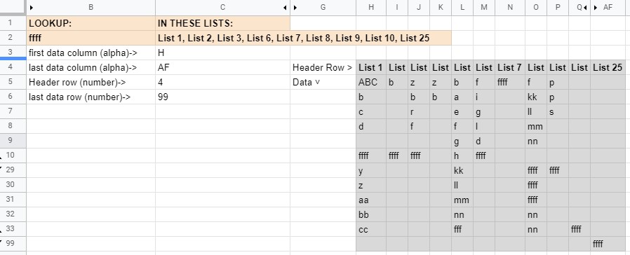
Refer to the image and enter the values for:

• first Column of data (alpha value),
• last Column of data (alpha value),
• first Row of data (the header row),
• last Row of data.
• All ranges in the formula are automatically calculated based on these four values.

FORMULA
The formula is:

=join(", ",QUERY({TRANSPOSE(indirect(C3&C5&":"&C4&C6))},"Select Col1 where "&JOIN(" or ",ARRAYFORMULA("Col"&(COLUMN(indirect((C3&C5+1)&":"&address(C5+1,C6+C5,4,true)))-COLUMN(indirect(C3&5))+1)&" = '"&$B$2&"'"))))

---

LOGIC

Query Data Range
TRANSPOSE(indirect(C3&C5&":"&C6&C7))

• the data range (H4:AF99) is built from the parameters in cells C3, C4, C5 and C6 (refer snapshot)
• the data is inserted using INDIRECT
• the data is transposed to that "Col1" contains the headers(the List#)

Where clause
where "&JOIN(" or ",ARRAYFORMULA("Col"&(COLUMN(indirect((C3&C5+1)&":"&address(C5+1,C6+C5,4,true)))-COLUMN(indirect(C3&5))+1)&" = '"&$B$2&"'"

• The purpose of this clause is to create a where condition like " where Col2 = 'ffff' or Col3 = 'ffff' or... Col96 = 'ffff'"
• Although there are only 25 Columns (H to AF) in the physical data, there are 96 Rows of data (including the header row).
• When the data is transposed (and rows become columns, and vice versa), there are 96 columns of data. "List#" occupies Col1, and data is in columns 2 to 96.
• Relative column numbers are generated by this snippet:
  • COLUMN(indirect((C3&C5+1)&":"&address(C5+1,C6+C5,4,true)))-COLUMN(indirect(C3&5))+1
  • which resolves to something like:
  • Column(H5:CY5)-Column(H5)-1
• when the JOIN function is added the outcome looks like this:
  • " where Col2 = 'ffff' or Col3 = 'ffff' or... Col96 = 'ffff'"
  • note the LAST column is #96

---

SAMPLE

• The data range in the sample is H4:AF99. Some columns and rows in the snapshot have been hidden
• The answer includes a value of "List25" because there is a value of "ffff" in Column 25 at row 99 (AF99).
  • The purpose of this cell value is to confirm that the formula evaluates every cell in the data range.
  • Other than the header, it is the only value in Column AF.

Answer 2

Formula

=JOIN(",", TOROW(BYCOL(H4:AF99, LAMBDA(c, 
    IFNA(INDEX(c, XMATCH(E1,c)>0)))), 1))

Functions

BYCOL BYROW IFNA INDEX JOIN LAMBDA TOROW XMATCH

_{Sample Screenshot (click to enlarge)}

Explanation

1. BYCOL passes each column from the range into a LAMBDA function one-by-one
2. LAMBDA assigns the name c to the current column passed in
3. LAMBDA's formula uses XMATCH to check if the lookup value in E1 can be located in c
4. Assuming XMATCH succeeds:
   • a number is returned matching the position of the lookup value in c.
   • Based on the height of the range H4:AF99, and excluding 1 (position of the heading) the number returned by a match would be from 2-95
   • Testing that the result is greater than zero XMATCH()>0 will return TRUE for any successful match.
     eg: 99>0=TRUE , 2>0=TRUE , etc.
   • This TRUE value is used as the row argument in INDEX to retrieve the header value.
   • This works because Sheets requires a number for INDEX's row argument and therefore converts TRUE to 1
   • INDEX(c,1) returns the header located in the first row of c
5. If XMATCH fails to locate the lookup value in c it returns a #N/A error.
   • This causes the functions that rely on the value to also return errors:
     #N/A>0=#N/A , INDEX(c,#N/A)=#N/A
   • IFNA is placed around the INDEX function without any additional argument to return an empty value instead of the error for each iteration of c where the lookup value isn't found.
6. BYROW returns an array that is a 25-column row where each cell is empty or contains a heading value.
7. The array is then placed in TOROW and its ignore empty cells argument is set to TRUE/1 which is a simple way to remove any empty cells in the row.
8. Remains only to JOIN the array of headings with the chosen delimiter.