What I'm trying to do is to highlight rows L to P in red if all cells say "False", and here is the formula I used:
=(sum(arrayformula(n(regexmatch($L2:$P2, "False")))) = 5)
This does not work unfortunately. I also tried the following formula (another way to put it) without any luck either:
=(sum(arrayformula(n(regexmatch($L2:$P2, "True|Unsure")))) = 0)
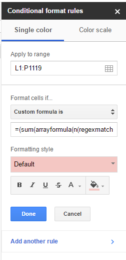
Next, is a snapshot of the conditional format rule:
Please help me figure out why the above formulas aren't working. If you need to see the sheet I'm working on, I've made a copy here.

