3

enter image description here

The title might sound confusing cause I don't know how to word it. Let start with the example

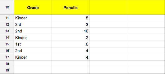
So I have a spreadasheet with data First column shows Grade levels: Kinder, First, Second, Third.... The other Column shows number of pencils for each grade.

I need a formula that selects only Kinder class and adds up all the pencils for them. Any ideas?

4
  • It is possible, the solution really depends on how your data is formatted. If you could add a screenshot or link to the spreadsheet it would be a lot easier to determine what exactly you are trying to do.
    – STowslee
    Commented Jan 18, 2017 at 19:48
  • I want to answer your question, but I'm confused about how you are using the words "row" and "column". A "row" is a horizontal set of "cells". A "column" is a vertical set of "cells". A "cell" is one rectangle, holding one value. So it doesn't make sense to say "Row A1". You would either say "Row 1" or "Cell A1", depending on what you mean. Also, it doesn't make sense to say "other rows in different columns", but you could say "other CELLS in different columns". It also may help you get better answers if you include a screenshot of your Google Sheet as an example. Commented Jan 18, 2017 at 19:59
  • I added a basic screenshot above. Basically I want a sum of pencils for Kinders only.
    – ben
    Commented Jan 18, 2017 at 20:06
  • I also must add, that spreadsheet always gets updated, so manually selecting rows from Pencil column and adding them up will not work.
    – ben
    Commented Jan 18, 2017 at 20:08

2 Answers 2

3

In the cell where you want to total, place this for the Kinder example:

=SUMIF(A11:A, "=Kinder", B11:B)

Since your grades are very limited, you could easily edit this for each case. Another option would be to reference the cell where Grade is defined:

=SUMIF($A$11:$A, "=" & D1, $B$11:$B)

In this example, you would place the formula in cell E1 and have Kinder in D1. You could then copy the formula down to other rows (E2, E3, etc) and have 1st, 2nd, etc in cells D2, D3, etc.

The $ in the Range tells the program to not increment that item when copying or moving the formula.

3
  • This is pretty handy for use in areas where pivot tables aren't an appropriate solution.
    – STowslee
    Commented Jan 18, 2017 at 22:43
  • Awesome, I love this. What if I want to calculate the sum for Kinders and 1st graders?
    – ben
    Commented Jan 18, 2017 at 23:13
  • 1
    @ben You would then use SUMIFS() which allows for multiple criteria: =SUMIF( $B$11:$B, $A$11:$A, "=Kinder", $A$11:$A, "=1st") and you can add additional criteria pairs to the end
    – Karl_S
    Commented Jan 19, 2017 at 2:39
1

Additionally you could use a pivot table to analyze each of the categories.

Data --> Pivot Table --> Select the range (SheetName!A:B)

Click on Rows (choose grade) Click on Values (choose pencils)

Your Answer

By clicking “Post Your Answer”, you agree to our terms of service and acknowledge you have read our privacy policy.

Not the answer you're looking for? Browse other questions tagged or ask your own question.