I think the answer from @twalbaum is fishing toward the right idea, but it can be improved by understanding in a little more detail the Google Sheets GOOGLEFINANCE() API which, in my opinion, is a little confusing. With some parameter combinations, it gives a scalar result and with other parameter combinations, it gives a range result.
Carefully reading the API, there are three or four use cases based on the attribute 2nd parameter provided.
attribute missing: returns a scalar real-time result- real-time data: You get real-time attributes if you use an
attribute value from the real-time set, including "price" and "priceopen".
- historical data: You get historical attributes if you use an
attribute value from the historical set, including "open" and "close".
- mutual fund data: You get mutual fund attributes if you use an
attribute from the mutual fund set, including "date" and "return152" among other oddities.
My answer will ignore the case of mutual fund data (as I haven't studied it, and the 2018 question is asking about GOOG which is not a mutual fund).
Now, the real-time API is where we get the last sold price, even if the market is closed. Incidentally, the date of the last sale can be displayed with googlefinance("GOOG", "tradetime").
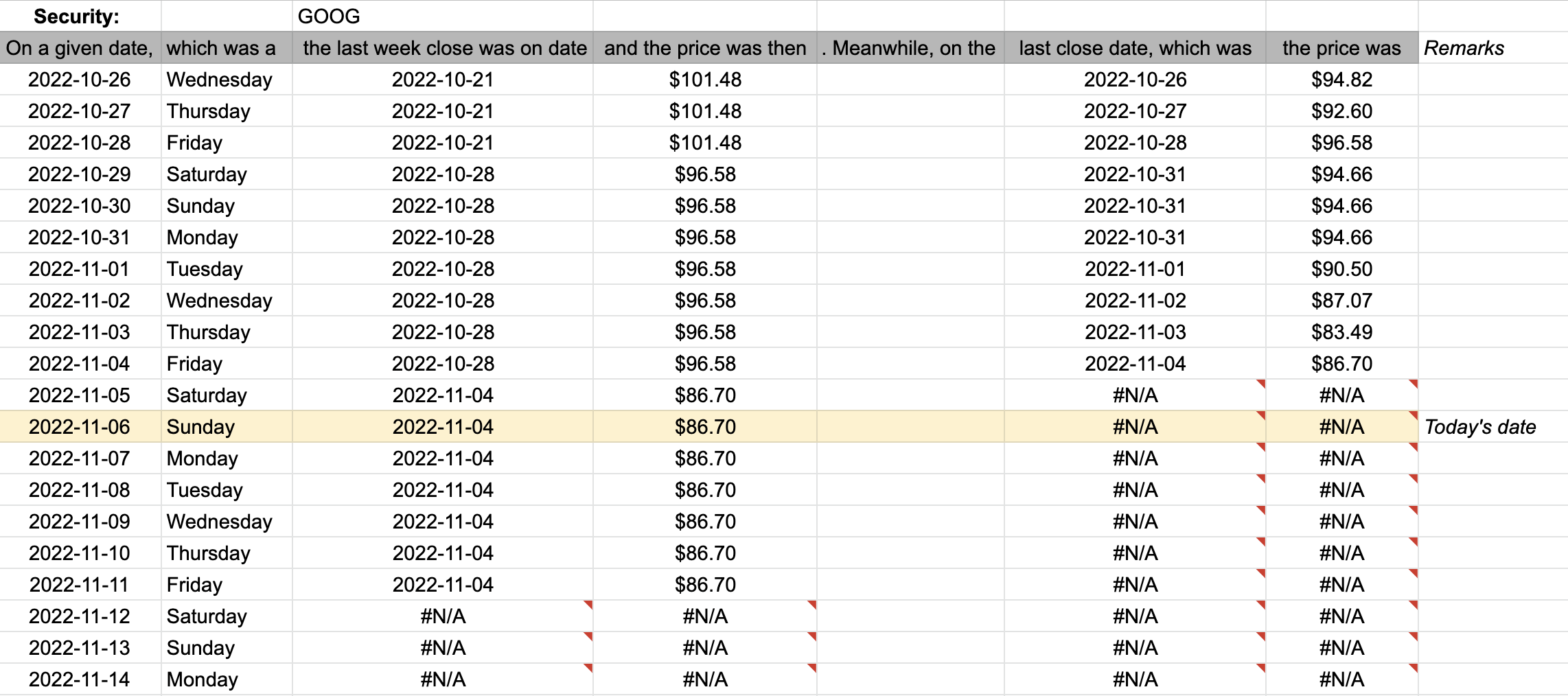
Meanwhile, going to historical data... if we specify most non-trading days the value comes back (apparently) as the close for the prior Friday. See below:

except, and I'm assuming this is a Google implementation bug, the closing value doesn't carry forward if the function is called on a non-trading day (columns F and G in the example).
However we can pull a nearly* equivalent value, the weekly close, by using the technique described by @twalbaum. See the result in columns C and D.
So I'd propose the solution is to conditionally return the daily close price, and if that happens to be #N/A, then to return the weekly close price.
=IFNA( index( googlefinance( "GOOG", "close", $DATE_CELL ), 2, 2 ), INDEX( googlefinance( "GOOG", "close", $DATE_CELL - 7, 7, "weekly" ), 2, 2 ) )
* Note, between cells D6 and G6 etc., the values differ by a small amount. I assume that's another Google error.
Conclusion: It seems like pulling the historical data from Google may be an inexact science. I'd propose my solution as a slightly more straightforward solution than the accepted solution.
Formulas:
- Column B:
=TEXT( A14, "WWWW" )
- Column C:
=INDEX( googlefinance( $C$1, "close", A14-7,A14, "weekly" ), 2, 1 )
- Column C:
=INDEX( googlefinance( $C$1, "close", A14-7,A14, "weekly" ), 2, 2 )
- Column E:
=INDEX( googlefinance( $C$1, "close", A14), 2, 1 )
- Column F:
=INDEX( googlefinance( $C$1, "close", A14), 2, 2 )

