1

This formula returns the daily stock prices of A1 in the last two years:

=GOOGLEFINANCE(A1,"Price",today()-(365*2),today(),"DAILY")

This formula returns the daily conversion rate from USD to EUR:

=GOOGLEFINANCE("Currency:USDEUR", "price", today()-(365*2),today())

I would like to put the two formulas together so that the historical stock prices are automatically given in EUR and not in USD. Is there any way to put the two formulas into one? Maybe with the help of SQL?

1 Answer 1

1

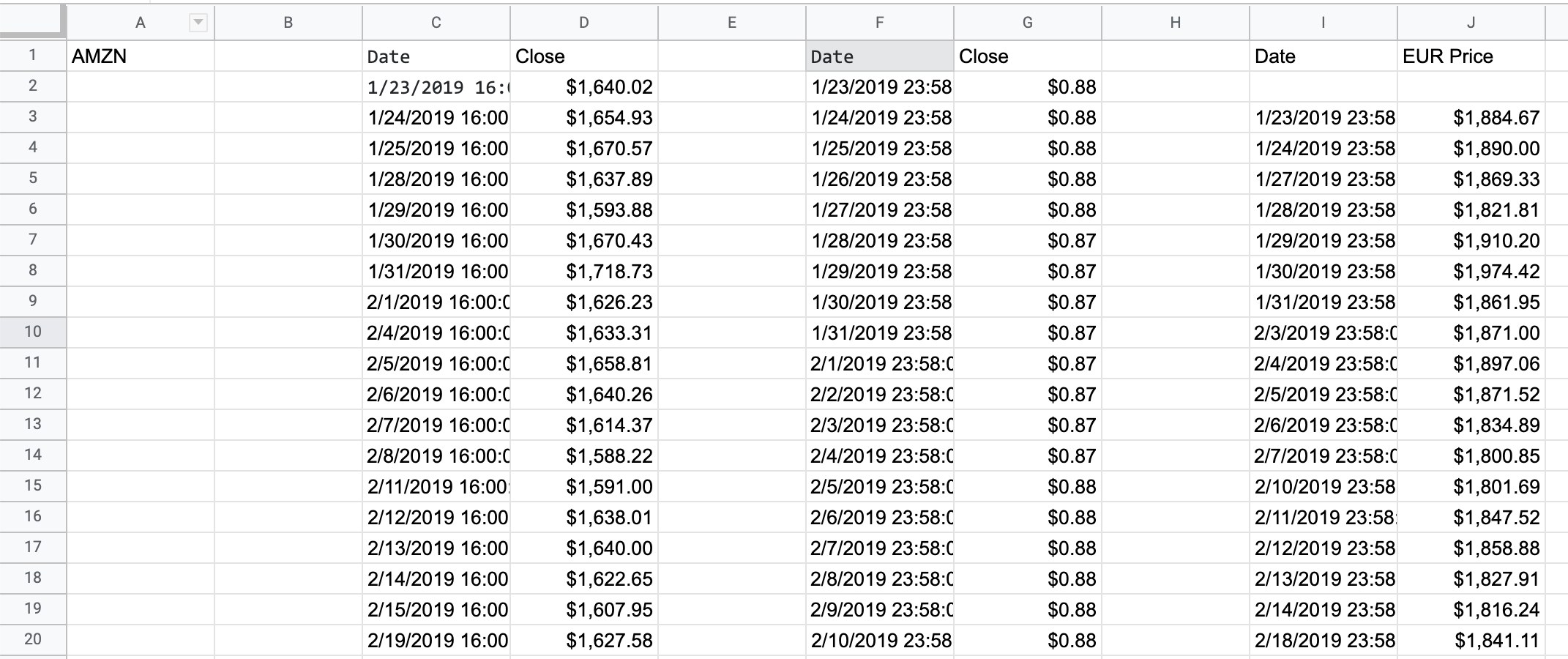
I took a stab at it here:

enter image description here

Column I has a formula like:

=QUERY({$F$2:$G$1000},"SELECT Col1 WHERE Col1 <= date'"& text(C3,"yyyy-mm-dd") &"' ORDER BY Col1 DESC LIMIT 1", -1)

This means that it pulls in the closest currency price date that's less than or equal to the stock price date.

Column J has a formula like:

=D3/VLOOKUP(I3, $F$2:$G$1000, 2, FALSE)

This means we're dividing the stock price by the currency conversion price on that nearest date. Hope this helps!

1
  • Hi! The formulas look good but I'm trying to use ONLY one formula that would do the job. For example: =ARRAYFORMULA(query(GOOGLEFINANCE(A1,"Price",today()-(365*2),today(),"DAILY"),"Select Col2 Order by Col1 DESC",0)*query(GOOGLEFINANCE("Currency:USDEUR", "price", today()-(365*2),today()),"Select Col2 Order by Col1 DESC",0)) This is almost OK, but the problem is that the dates stocks historical dates and exchange rates are soon offset. Any way to improve it? Commented Jan 22, 2021 at 21:30

Your Answer

By clicking “Post Your Answer”, you agree to our terms of service and acknowledge you have read our privacy policy.

Not the answer you're looking for? Browse other questions tagged or ask your own question.