0

Beforehand please check my sample sheet.

I'm trying to use SUMIF or any specific formula that shows the total amount of income of each month over on the side (March, April, May...)

As noticed the date (month) is not always the same on each column (Date 1, Date 2, Date 3...), it may vary.

I've tried SUMIF, FILTER, ARRAYFORMULA, but haven't had any luck.

Is there any way to do this or do I have to change the whole structure?

2
  • so basically you want to dissect it per each month and sum it up right?
    – user0
    Commented Jul 11, 2018 at 19:15
  • Yes. Basically sum all the amounts from Payments - range or columns (E:E, G:G, I:I, K:K M:M, O:O) that match the month MARCH looked up on each of the colums of Dates (F:F, H:H, J:J, L:L, N:N, P:P)
    – A. C.
    Commented Jul 11, 2018 at 20:20

2 Answers 2

0

S2:

=ARRAYFORMULA(SUMIF(TEXT($F$2:$P$5,"mmmmyyyy"),S$1&"2018",$E$2:$O$5))

Drag to right.

SUM E2:O5,IF F2:P5 has S1's Month&2018.

1
  • Wow. This actually worked! I really appreciate it!
    – A. C.
    Commented Jul 12, 2018 at 13:40
0

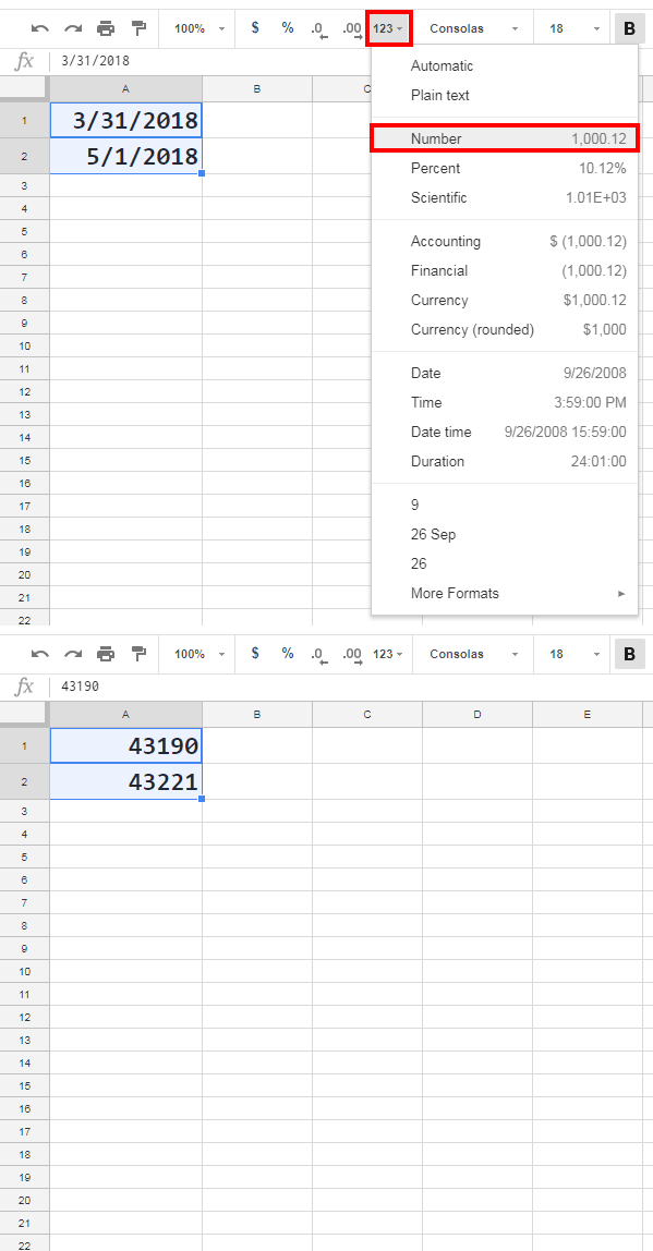
First, you need to convert a date to a number and find out the range of the month in numbers.

March starts with the end of 28th Feb, and ends with the start of 1st Apr, therefore:

  • 02/28/2018 converted to a number is 43159
  • 04/01/2018 converted to a number is 43191
  • so now we know that we need to filter out stuff between 43159 - 43191 and sum it

TOTAL PER ROW PER MONTH:

(paste it into cell S2 and drag it down)

=SUM(IF(COUNTIFS(F2 < 43159, F2 > 43191),SUM(E2,
     IF(COUNTIFS(H2 < 43159, H2 > 43191),SUM(G2,
     IF(COUNTIFS(J2 < 43159, J2 > 43191),SUM(I2,
     IF(COUNTIFS(L2 < 43159, L2 > 43191),SUM(K2,
     IF(COUNTIFS(N2 < 43159, N2 > 43191),SUM(M2,
     IF(COUNTIFS(P2 < 43159, P2 > 43191),SUM(O2)))))))))))))

TOTAL PER ALL ROWS PER MONTH:

(paste it into cell S2)

=SUM(IFERROR(FILTER((E2:E5),MONTH(F2:F5)=3),),
     IFERROR(FILTER((G2:G5),MONTH(H2:H5)=3),),
     IFERROR(FILTER((I2:I5),MONTH(J2:J5)=3),),
     IFERROR(FILTER((K2:K5),MONTH(L2:L5)=3),),
     IFERROR(FILTER((M2:M5),MONTH(N2:N5)=3),),
     IFERROR(FILTER((O2:O5),MONTH(P2:P5)=3),))
5
  • I applied it to the main document and it's giving me a number that's not correct. I did however try =SUM(FILTER((E2:E5),MONTH(F2:F5)=3)) and was giving me the correct one, however I cannot deploy MONTH to take into account other columns.
    – A. C.
    Commented Jul 11, 2018 at 21:33
  • @A.C. fixed. try now
    – user0
    Commented Jul 11, 2018 at 22:00
  • Still gave me an error on the main document.
    – A. C.
    Commented Jul 12, 2018 at 13:41
  • @A.C. cant be. see yourself: docs.google.com/spreadsheets/d/…
    – user0
    Commented Jul 12, 2018 at 13:51
  • 1
    Got it! It also worked. Appreciate it! :)
    – A. C.
    Commented Jul 12, 2018 at 16:46

Your Answer

By clicking “Post Your Answer”, you agree to our terms of service and acknowledge you have read our privacy policy.

Not the answer you're looking for? Browse other questions tagged or ask your own question.