Google Sheets Conditional Formatting

Question

I am trying to make a certain cell on my sheet light up based on what week it is.

Each cell contains the value Week X where the X is a week-number.

After a little bit of experimentation I have made the following:

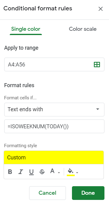
Here the cells A4:A56 are the cells with Week X in them.

I want each one each week to light up in beautiful yellow based on the week, but instead, this does nothing (no cells turn yellow).

Is there any way I can get my desired result with conditional formatting in Google Sheets?

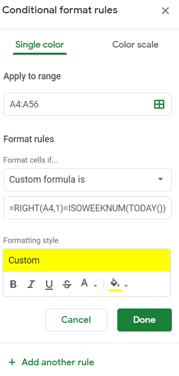
Update (an attempted answer made by Rubén, did not work):

Add sample data to the question and a link to a demo spreadsheet shared with anyone with the link can view. — Rubén - Volunteer Moderator -, Commented May 17, 2019 at 15:03

user0 · Accepted Answer · 2019-05-18 23:39:06Z

1

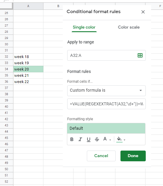
=VALUE(REGEXEXTRACT(A4,"\d+"))=WEEKNUM(TODAY(),2)

answered May 18, 2019 at 23:39

user0

27.1k10 gold badges53 silver badges78 bronze badges

1

Works perfectly, thank you very much!
– ViRALiC
Commented May 20, 2019 at 7:28

Add a comment |

Rubén - Volunteer Moderator - · Accepted Answer · 2019-05-16 13:54:17Z

0

To use a formula for conditional formatting, instead of Text ends with select Custom Formula.

Then use a formula like the following

=RIGHT(A4,1)=ISOWEEKNUM(TODAY())

answered May 16, 2019 at 13:54

46.1k18 gold badges100 silver badges297 bronze badges

I attempted your solution but no change was made to any cells, sadly. Did I make a mistake?
– ViRALiC
Commented May 17, 2019 at 14:17

Add a comment |

2 Answers 2