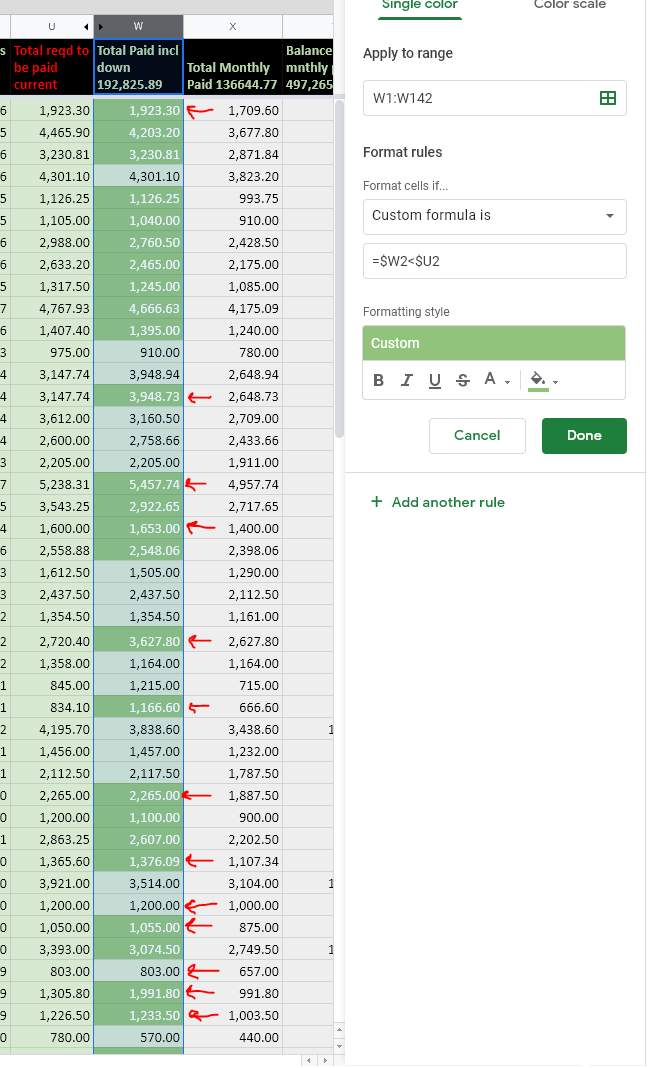
I recently tried to edit the conditional formatting for a column that was working correctly before and then change it back to the same exact formula it had before and now it isn't working correctly. The formula is =$W2<$U2 but it appears to be ignoring the less than the part. It highlights cells that are equal to and greater too as well. Both columns are formatted to numbers. I'm not sure why it worked before and doesn't want to work now. I tried completely deleting the conditional formatting and starting over. Same thing. Any ideas what the problem is?
Add a comment
|
1 Answer
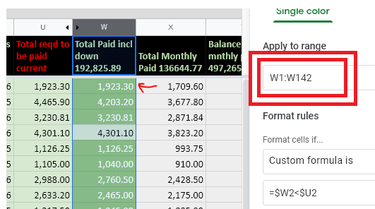
Looks like your Conditional Formatting is offset by 1 row because you applied it to range W1:W142 instead of W2:W142
-
1Awesome, thank you! I was staring at that for about an hour trying to figure out what was wrong. Commented Jul 25, 2019 at 17:59


