Copy/multiply cell contents based on number in another cell

Question

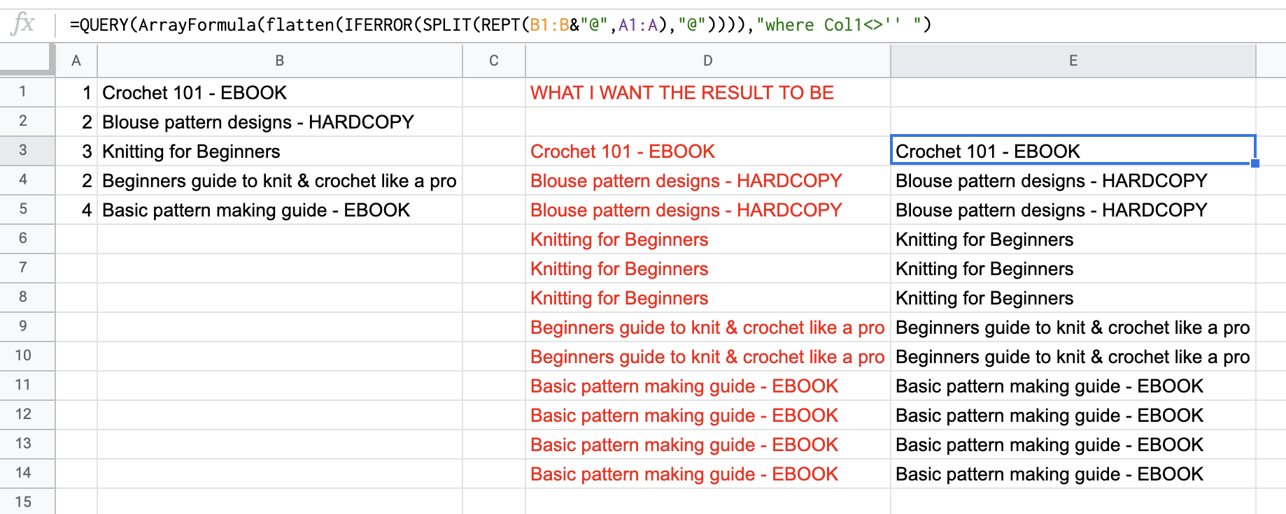
I have a list of items, Col. B & numbers in Col. A. I want to multiply/copy the text in cell B based on the number in their relative cell A. I.e. multiply 'B' by the number of times in 'A'

Here's the sample spreadsheet:https://docs.google.com/spreadsheets/d/1_jbgugr93t6CYY08Bi83SH3pWJIH8B1ukfCKiPwtt4M/edit?usp=sharing

I've also shown in Col. D in red, what I envision as my result would look like. Right now I do this manually, copy the contents the relevant number of times.

Is there a way to do this faster.

Answer 1

Please use the following

=QUERY(ArrayFormula(flatten(IFERROR(SPLIT(REPT(B1:B&"@",A1:A),"@")))),"where Col1<>'' ")

How the (undocumented) flatten function work.
When we use flatten on an array of cells, it transposes the array row by row into a single column.

Please notice the difference between flatten and TRANSPOSE

+------+-----+----+-----------------+----------+----------+
| array of cells  | =flatten(A1:C2) |  =TRANSPOSE(A1:C2)  |
+------+-----+----+-----------------+----------+----------+
|   1  |  2  |  3 |        1        |     1    |     4    |
|   4  |  5  |  6 |        2        |     2    |     5    |
|      |     |    |        3        |     3    |     6    |
|      |     |    |        4        |          |          |
|      |     |    |        5        |          |          |
|      |     |    |        6        |          |          |
+------+-----+----+-----------------+----------+----------+

Functions used:

• QUERY
• ArrayFormula
• IFERROR
• SPLIT
• REPT

Answer 2

Here is another approach:

=ArrayFormula(VLOOKUP(TRANSPOSE(SPLIT(JOIN("",REPT(ROW(A:A)&"@",A:A)),"@",0,1)),{ROW(A:A),B:B},2,FALSE))

How It Works

=ArrayFormula(...) signifies that the formula will process an entire range and not just one cell.

Now, working from the inside out...

REPT(ROW(A:A)&"@",A:A) will add the @ symbol onto the end of each row number and then repeat that string however many times is listed in A:A. For instance, if row 1 Column A indicates to repeat 1x, the string for that row will be 1@. If row 2 Column A indicates it is to repeat 2x, the sting for that row will be 2@2@.

JOIN("",...)

All of those strings will be joined into one long string (e.g., 1@2@2@3@3@3@...)

SPLIT(...,"@",0,1)

That long string will be split apart at the @ symbol into a long virtual row of individual numbers, e.g.:

1 2 2 3 3 3...

TRANSPOSE(...)

That long virtual row of individual numbers will be transposed into a column of the same numbers, e.g.:

1

2

2

3

3

3

etc.

VLOOKUP(...,{ROW(A:A),B:B},2,FALSE))

Each of those individual numbers in the column will be looked up within a virtual array composed of all row numbers in column one and all B:B text in column two. When each exact match is found (signified by FALSE), the Column 2 data will be returned.