Google Sheet Formula Error

Question

Hoping to get a little help with a formula I am making I have used it in other columns to calculate an outcome, but for some reason when I go to decimals under 0 it give me a #N/A "No Match".

Here is my goal.

• .049 and under will be given a 0
• .05 to .99 will be given a 1
• .1 to .19 will be given a 2
• .2 and above will be given a 3

The formula pulls from three different cells then adds the given number for each up.

Here is the formula I have that I have used in other columns with success.

=sum(IFS(AND(BB3>=0.05,BB3<=0.09),1,AND(BB3>=0.1,BB3<=0.19),2,OR(BB3>=0.2),3,OR(BB3<0.049),0)+IFS(AND(AZ3>=0.05,AZ3<=0.09),1,AND(AZ3>=0.1,AZ3<=0.19),2,OR(AZ3>=0.2),3,OR(AZ3<0.049),0)+IFS(AND(AX3>=0.05,AX3<=0.09),1,AND(AX3>=0.1,AX3<=0.19),2,OR(AX3>=0.2),3,OR(AX3<0.049),0))

I should mention that I am pulling the numbers from a column that is taking the different between two numbers pulled from another sheet within the document. (I know full number inception) Cell BC3 is where I have been working.

Here is a link to the document I have been working on: https://docs.google.com/spreadsheets/d/1itmmnjydelvqw8oYnOQ6IEFCJEqrn79KerRzwpEBN6k/edit?usp=sharing

Answer 1

In addition to the problem with the score in BC3, the formula involves duplication to the extent that it is prone to error AND makes any change in rates a major undertaking. This answer provides a more simple alternative.

Step#1 - Create a table of scores

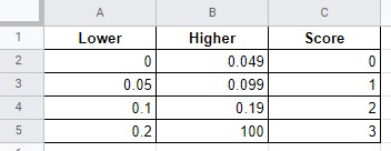
Create a table with the respective low scores, high scores, and point values.

Step#2 - Modified formula based on VLOOKUP

Use this formula in cell BC3: =sum(vlookup(BB3,score_analysis!$A$2:$C$5,3,true)+vlookup(AZ3,score_analysis!$A$2:$C$5,3,true)+vlookup(AX3,score_analysis!$A$2:$C$5,3,true))

Copy the formula down as many rows as their is data.

Answer 2

An observation about the formula in BC3

When the sub-totals of raw values are used, the formula fails.

When the sub-totals are rounded, the formula works.

I don't have a full understanding of how the values in "results sheets" are entered or obtained, but rounding does appear to a be a solution that should solve the problem.

---

Background

• The formula in BC3 is the SUM of three IFS formula

  • The IFS relate to Columns "BB", "AZ" and "AX" respectively.

• At face-value the result in cell BC3 should be 5

  • BB = 2
  • AZ = 2
  • ZX = 1
  • Total = 5

• However, the calculations for AZ and AX are failing.

  • Both these columns have a value of 0.1 which should generate a result of 2

• The values in the respective "results sheets" appear to be hand-entered and are numbers, so there is no obvious reason why these formula should fail.

Rounding results

• As a test, on Row 4 I created formulas that round the results from row3 in Column AX, AZ, and BB. The rounding was to 3 decimal places.
  • =round(AX3,3)
  • =round(AZ3,3)
  • =round(BB3,3)

When this is done, the formula in Column BB calculates the correct result.

---

Sample