Can't sort correctly with thousand separator

Question

I'm making a list to compare who's leading the "most watched films" race, using IMPORTXML() to scrap information from Letterboxd and SORT().

The thing is that Letterboxd uses commas as thousand separator, and SORT() thinks it is a decimal separator. Because of this, it puts the highest number down below the list when sorted. I tried using the =SUBSTITUTE() function (=SUBSTITUTE(IMPORTXML(A3; "//*[@id='profile-header']/div/div[4]/div[1]/h4[1]/a/span[1]"); ","; ".")) for changing commas to dots (or even removing commas) and it doesn't work. =SORT() (=sort(D3:E21; 2; FALSE)) sorts not by highest number, it does something strange like this: 95, 9, 87, 82, 7, (...) 1302, 12

What can I do? Changing locale does not work.

Answer 1

Curiosity is a dangerous thing. @Daniele asked what is the url you wrote in A3? and I thought, that's a good question cause the xpath and the URL kind-of go together. So I got carried away and this is the result.

Note: the results are formulas based on the original IMPORTXML. At some stage, one might wish to Copy, Paste special, Values only to convert any given result to a value.

Some variables

---

ImportXML

Cell A7: =transpose(importxml(B1;B2))

This generates the following data (or at least this snapshot of the first 20 values). Note: this formula uses a semi-colon separator because that's what the OP uses.

BTW, since it is a list, you could probably/possibly (warning: untested assertion) use IMPORTHTML() (along with the right query and index).

---

Results

The results are broken into data elements; you could combine these into just four formula (Score, Name, Year and Rating) if you were so inclined.

• Length of the imported string: =arrayformula(len(A7:A106))
• Position/location of the decimal point: =arrayformula(search($B$3;A7:A106))
• Position/location of the first star (★): =arrayformula(search($B$4;A7:A106))
• Number of Stars: =arrayformula((LEN(A7:A106)-LEN(SUBSTITUTE(A7:A106;$B$4;)))/LEN($B$4))
• Number of 'Halfs' (½): =arrayformula((LEN(A7:A106)-LEN(SUBSTITUTE(A7:A106;$B$5;)))/LEN($B$5))
• Score (out of 100): =arrayformula(value(left(A7:A106;D7:D106-1)))
• Title/Name : =arrayformula(if(iserr(E7:E106);mid(A7:A106;D7:D106+1;C7:C106-D7:D106-5-1);mid(A7:A106;D7:D106+1;E7:E106-D7:D106-1-6)))
• Year: =arrayformula(if(iserr(E7:E106);right(trim(A7:A106);4);mid(A7:A106;E7:E106-5;4)))
• Rating: =arrayformula(if(F7:F106=0;"";rept($B$4;F7:F106))&if(G7:G106=0;"";rept($B$5;G7:G106)))

Answer 2

The IMPORTHTML version

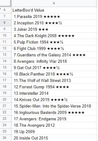
I mentioned in my other answer that the data could be obtained using importhtml. Well...

Note: Again, the results are formulas based on the original IMPORTHTML formula. At some stage, one might wish to Copy, Paste special, Values only to convert any given result to a value.

Some variables

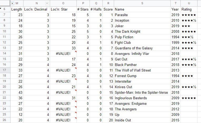
Note that this version doesn't search for the star ("★") or half ("½") characters. This is because the format generated by importhtml is completely different to the importxml format.

IMPORTXTML Format >

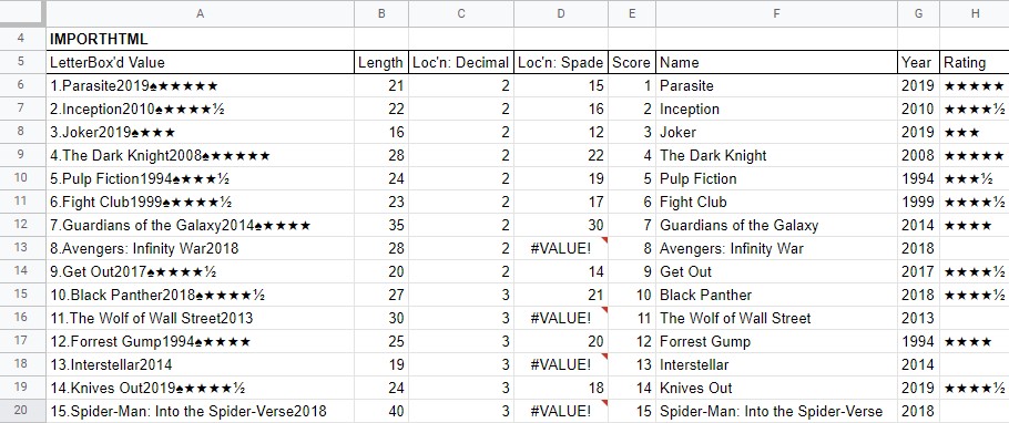
Records with a rating (such as 'Guardians of the Galaxy') include 2 (two) carriage returns; records without a rating (such as 'Avengers: Infinity War') don't have any carriage returns.

So the spade character ('♠️') is used (substitute) to identify those records with a rating and those without a rating.

---

ImportHTML

Cell A6: =arrayformula(SUBSTITUTE(SUBSTITUTE(importhtml($B$1;"list";14);char(10);"";1);char(10);"♠️";1))

This generates the following. Note: again this formula uses a semi-colon separator because that's what the OP uses.

---

Results

The results are broken into data elements (similar to the IMPORTXML results). But this time, I've built single formulas for the 'Score', 'Name', 'Year' and 'Rating' and I'll show just those.

• Score (out of 100): =arrayformula(value(left(A6:A105;search($B$2;A6:A105)-1)))
• Title/Name : =arrayformula(if(iserr(search($B$3;A6:A105));mid(A6:A105;search($B$2;A6:A105)+1;len(A6:A105)-search($B$2;A6:A105)-4);mid(A6:A105;search($B$2;A6:A105)+1;search($B$3;A6:A105)-search($B$2;A6:A105)-1-4)))
• Year: =arrayformula(if(iserr(search($B$3;A6:A105));right(A6:A105;4);mid(A6:A105;search($B$3;A6:A105)-4;4)))
• Rating: =arrayformula(if(iserr(search($B$3;A6:A105));"";mid(A6:A105;search($B$3;A6:A105)+1;len(A6:A105)-search($B$3;A6:A105))))