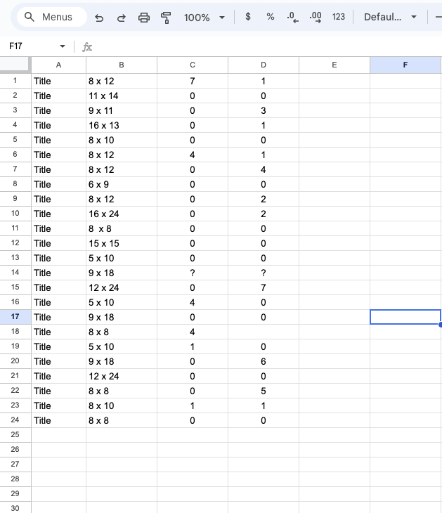
I'm trying to create a rule that will turn cells A through D red if cells C and D equal 0 or less.
I know how to make the rule with just one cell equaling 0, but would like to make it conditional on both equaling zero.
I'm trying to create a rule that will turn cells A through D red if cells C and D equal 0 or less.
I know how to make the rule with just one cell equaling 0, but would like to make it conditional on both equaling zero.
Use this conditional formatting custom formula rule for the range A1:D:
=isnumber($C1) * (max($C1:$D1) <= 0)