Query based on column header in Google Sheets

Question

I am trying to automate Worship list using Google Sheets, so it works good but one thing I can't do can be more than useful.

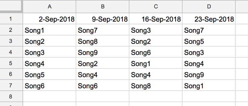
I have a sheet like this:

in row 1 dates and below songs used that Sunday.

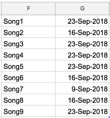
As a result, I need the table like this, where I can see when the song was used last time:

MATCH works good with one column, but how can I do it with multi-column range?

I've also tried to join columns to strings:

=join(",",A2:A7)

And then use QUERY:

=query(A$12:B$15,"select max(A) where B like '%"&F1&"%' label max(A) ''")

And it works, but not automatically...

Answer 1

I created a sample sheet from your data, with a few more columns.

Basically, I took raw data, and added another row immediately underneath the date header. This new row contains =JOIN(";",A4:A9), and is copied to each cell in the row.

To produce the desired output, I simply did an HLOOKUP on the dates and the joined data (with a SORT to put it in the correct order). Here is the formula I used:

=HLOOKUP("*"&D12&"*",TRANSPOSE(SORT(TRANSPOSE($A$2:$G$3),2,FALSE)),2,FALSE)

D12 contains "Song1" in this case. A2:G3 contains the dates and the songs joined together.

I'm sure there are better methods to accomplish what you want, especially ones which don't require copying multiple formulas to a lot of cells. I just did this as a quick proof of concept.