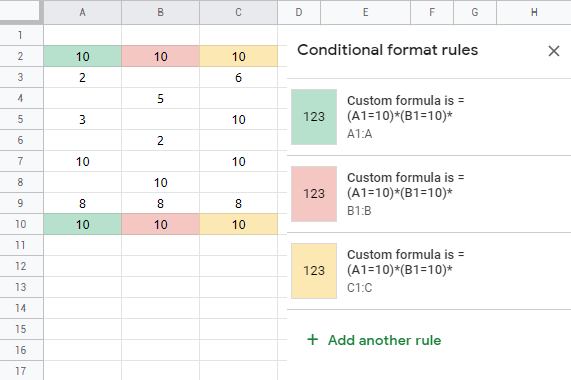
I have a Google spreadsheet with arbitrary data. Three adjacent columns (let's say A, B and C) have been set up with Data Validation to only allow values from 1 to 10.
I'm looking for a way to validate that if all three columns of a single row (e.g. A4, B4 & C4) have a value of 10, all three cells should get formatted differently, let's say a different background color for the sake of simplicity.
This formatting should apply to an entire range from A1/B1/C1 to A300/B300/C300, and here lies the problem.
I've tried many ways to do this with data validation, built-in functions and conditional formatting, but other than going row by row applying the formatting, I haven't found an actually effective way to do this. Had to resort to the script editor and write a function called when onEdit() gets triggered, but this is slow and the coloring can actually be seen being applied when the code triggers because each row needs to be checked individually.
Is there any way to do this without having to resort to scripting, and without having to do it row by row?

