Dynamic Master sheet that grabs red formatted cells from another sheet

Question

The title may be a little too ambiguous but I'll try to give a rundown as best I can;

I have a Google sheet with multiple "Sheets" or Tabs (as I'd like to call them) within it.

The Main tab is blank and the rest have various cells with different dates on them. The dates that are close turn their respective cells Red. I have existing conditional formatting to do this.

What I want to achieve is the main tab basically checks all the other tabs for any red cells and pops them into the main sheet in a vertical column.

Here's an example:

"Second tab"

• (A1) Date 1 (green)

• (A2) Date 2 (red)

• (A3) Date 3 (red)

• (A4) Date 4 (Green)

"Main tab"

• (A1) Date 2 (red)

• (A2) Date 3 (red)

As you can see, "Main tab" ignores any green cells from "Second tab" and only grabs the red ones. In my case though, there are many more tabs, not just 1.

I have a feeling =IMPORTRANGE may help in this scenario? Maybe.

Any help is greatly appreciated!

Answer 1

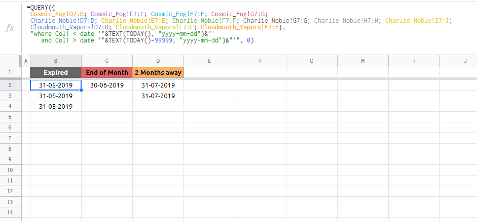
You don't need IMPORTRANGE. Also, you can't have a formula that checks only for color (you would need a script or addon for that). However, you mention that you already have conditional formatting rules in place that already do their job to turn cells red so you can gain an advantage of it and use the same rules in your Main sheet (but not as CF) to get data you need.

---

• paste in B2 cell:

=QUERY({
 Cosmic_Fog!D7:D; Cosmic_Fog!E7:E; Cosmic_Fog!F7:F; Cosmic_Fog!G7:G; 
 Charlie_Noble!D7:D; Charlie_Noble!E7:E; Charlie_Noble!F7:F; Charlie_Noble!G7:G; Charlie_Noble!H7:H; Charlie_Noble!I7:I; 
 Cloudmouth_Vapors!D7:D; Cloudmouth_Vapors!E7:E; Cloudmouth_Vapors!F7:F}, 
 "where Col1 < date '"&TEXT(TODAY(), "yyyy-mm-dd")&"' 
    and Col1 > date '"&TEXT(TODAY()-99999, "yyyy-mm-dd")&"'", 0)

• paste in C2 cell:

=QUERY({
 Cosmic_Fog!D7:D; Cosmic_Fog!E7:E; Cosmic_Fog!F7:F; Cosmic_Fog!G7:G; 
 Charlie_Noble!D7:D; Charlie_Noble!E7:E; Charlie_Noble!F7:F; Charlie_Noble!G7:G; Charlie_Noble!H7:H; Charlie_Noble!I7:I; 
 Cloudmouth_Vapors!D7:D; Cloudmouth_Vapors!E7:E; Cloudmouth_Vapors!F7:F}, 
 "where Col1 > date '"&TEXT(TODAY(), "yyyy-mm-dd")&"' 
    and Col1 < date '"&TEXT(TODAY()+30, "yyyy-mm-dd")&"'", 0)

• paste in D2 cell:

=QUERY({
 Cosmic_Fog!D7:D; Cosmic_Fog!E7:E; Cosmic_Fog!F7:F; Cosmic_Fog!G7:G; 
 Charlie_Noble!D7:D; Charlie_Noble!E7:E; Charlie_Noble!F7:F; Charlie_Noble!G7:G; Charlie_Noble!H7:H; Charlie_Noble!I7:I; 
 Cloudmouth_Vapors!D7:D; Cloudmouth_Vapors!E7:E; Cloudmouth_Vapors!F7:F}, 
 "where Col1 > date '"&TEXT(TODAY()+29, "yyyy-mm-dd")&"' 
    and Col1 < date '"&TEXT(TODAY()+61, "yyyy-mm-dd")&"'", 0)

---

• if you want to get rid of duplicates wrap each query into UNIQUE