2

I'm trying to create a formula that will allow all the cells in Column B to include a hyperlink to cells in Column J in their corresponding rows. The kicker is that I'm trying to keep the current values of the cells in Column B as the title of the hyperlink.

I've been trying different iterations of:

=HYPERLINK(CONCATENATE("<link_from_column_j_cell>",B2);B2)

but it doesn't appear to function the way I've intended.

Any thoughts or advice would be appreciated.

UPDATE:

Using the advice provided by marikamitsos, I was able to adjust my formula to something very close to what I am looking for, but it still isn't the exact behavior I'm trying to achieve.

=ArrayFormula(HYPERLINK("https://docs.google.com/spreadsheets/d/1znqvu-nWk_0rBzudQm5PymyLlWsuEJTrmPqbhm4g6CI/edit#gid=0&range=J2:J632",K2:K632))

This array formula pulls names from one column, and then embeds a hyperlink to the entire range of descriptions. However, the link does not direct you to the corresponding cell containing the description for the exact item.

HYPERLINK("https://docs.google.com/spreadsheets/d/1znqvu-nWk_0rBzudQm5PymyLlWsuEJTrmPqbhm4g6CI/edit#gid=0&range=J2",K2)

produces the correct behavior, but only for a single cell in the name range. Due to there being 632 entries, I was hoping that a proper ArrayFormula could provide and iterative range, so that K2 links to J2, K3 to J3 and so forth. Any further clarification on syntax would be greatly appreciated. Or, if I'd be better off with a macro or script.

0

1 Answer 1

1

Edited following OP's request:

How to create no pop-up Hyperlinks/Bookmarks for an array of cells within the same tab/sheet

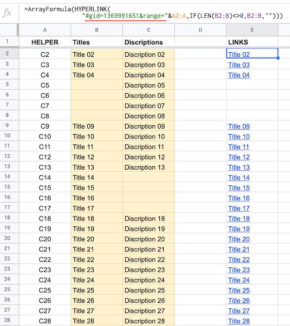
=ArrayFormula(HYPERLINK( 
                "#gid=1369991651&range="&A2:A,IF(LEN(B2:B)<>0,B2:B,"")))

You will need a helper column placed anywhere within the same tab and in this column you will reference the cells of your "Descriptions" column. You can then, even hide the "HELPER" column.

Notice that because we reference an array within the same tab/sheet we do NOT need the sheet ID. Instead we use the # character.

The created hyperlinks behave like HTML "anchors" and do not produce any pop-up windows.

How to create no pop-ups Hyperlinks/Bookmarks for an array of cells within the same tab/sheet


Original answer:

Assuming your text/title is in cell B2 the formula you need is:

=HYPERLINK("http://www.google.com/";""&B2&"")

If you want to use an ARRAYFORMULA you would change the above formula to:

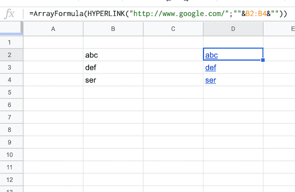
=ArrayFormula(HYPERLINK("http://www.google.com/";""&B2:B4&""))

enter image description here

When you want to have the formula link different cell titles to consecutive link cells (of the same row or not) you can use:

=ArrayFormula(HYPERLINK((""&C21:C24);B21:B24))

7
  • Awesome! This definitely seems like a step in the right direction. I'm still learning many of the intricacies in Google Sheets/Excel, so forgive my ignorance. Here is an image of the sheet I have been working on. I have been making modifications to an existing spreadsheet to make a gaming tool for my group on Discord. The goal is to keep the text already in the cells under column B, but have the text hyperlink to a cell in column J on the same row. Because of existing formulas and formatting on this worksheet, I'm avoiding adding/removing rows. Commented Feb 4, 2020 at 1:47
  • In other words, I want the <name> in B2 to hyperlink to the description in J2. B3 to J3, and so on. Commented Feb 4, 2020 at 1:49
  • Please check the updated answer. Commented Feb 4, 2020 at 2:34
  • Thank you for the update! So my new formula looks like this "=ArrayFormula(HYPERLINK(J2:J632,K2:K632))" But the link it embeds to the text doesn't actually work. It produces links like this: "for%20one%20hour%2C%20the%..." which just open a new blank tab. Commented Feb 4, 2020 at 3:10
  • Thank you so much for your time and effort in explaining this to me! This solution produces the EXACT behavior I've been looking for! Thank you for all of your help and patience, you are a lifesaver! Commented Feb 5, 2020 at 21:06

Your Answer

By clicking “Post Your Answer”, you agree to our terms of service and acknowledge you have read our privacy policy.

Not the answer you're looking for? Browse other questions tagged or ask your own question.