How to use HYPERLINK text as the first argument for MATCH?

Question

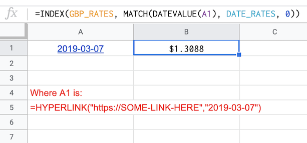
I have one column with hyperlinks and another column in which I do a vertical lookup using INDEX + MATCH. The catch is that the first argument for the MATCH function should be the correspondent value on the first column.

The problem is that it doesn't work because of the hyperlinks. If I remove them and leave the values as plain texts, it works.

I did some research and found that I can use the following formula to get the text value from a hyperlink cell:

=””&

Which works indeed if used like that, but not when it's the first argument of MATCH:

=INDEX(GBP_RATES, MATCH(""&A8, DATE_RATES, 0))

I get the following error:

#NAME?

Is there any workaround other than decoupling the text from the ULR into two different columns?

Answer 1

In your spreadsheet the issue is that the hyperlink as well as your named range DATE_RATES are dates.
In this case you do not need the & but the DATEVALUE function.

Please use the following formula:

=INDEX(GBP_RATES, MATCH(DATEVALUE(A1), DATE_RATES, 0))

Functions used:

• DATEVALUE
• MATCH
• INDEX