0

I am a beginner with code and formulas here, so I was wondering if anyone could do exactly what was done on this question:

Trying to use Google Sheets importHTML() to import a table. It forces content to a date format

to this table:

https://www.actionnetwork.com/nfl/nfl-against-the-spread-standings

In short, IMPORTHTML changes sports records to date format. Changing the numbers format to plain text does not work when importing websites, as the format is preset. However, there is a workaround using the ARRAYFORMULA and REGEXREPLACE. When you open the link scroll down to Aurielle's response for the single formula version. I have tried to implement the workaround for the NFL record link above, but I can't quite find the right formula mostly because, again, I'm a beginner and I don't understand these formulas. I was wondering if anyone understood this better and could give me the correct formula for this specific table of NFL records.

I would greatly appreciate any help!

1
  • 1
    Welcome. Just to point out something a substantial difference between the data on "actionnetwork.com/nfl/nfl-against-the-spread-standings" and the referenced "sportsnet.ca/hockey/nhl/standings". In your data, a result of x-y-z is the except to the rule; most results are x-y. Compare this to the referenced site, columns 11 and 12 contain the results and in every case, the results are x-y-z. In short, @Aurielle combination of arrayformula(REGEXREPLACE(query(text(IMPORTHTML is ingenious, but it produces patchy results for your URL.
    – Tedinoz
    Commented Nov 22, 2020 at 4:26

3 Answers 3

2

There are likely to be many solutions to your question. Even in this answer, I would expect that the structure could be simplified - possiblky along the lines of the answer by Rubén in Trying to use Google Sheets importHTML() to import a table. It forces content to a date format. In that answer, Rubén constructed a formula in which column() was a variable. This would be a convenient enhancement to this answer.

The answer is in two parts:

  • Part#1 - variables

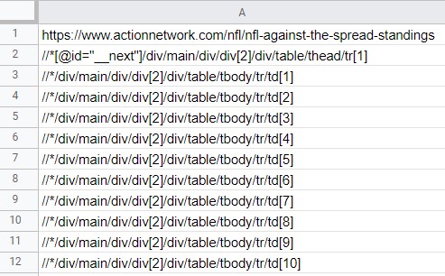
    • Cell A1: the URL https://www.actionnetwork.com/nfl/nfl-against-the-spread-standings
    • Cell A2-A12 - (11 cells) contain the XPath for specific elements of the output formulae.
      • A2-Headers: //*[@id="__next"]/div/main/div/div[2]/div/table/thead/tr[1]
      • A3-Team Names: //*/div/main/div/div[2]/div/table/tbody/tr/td[1]
      • A4-Overall: //*/div/main/div/div[2]/div/table/tbody/tr/td[2]
      • A5-Home: //*/div/main/div/div[2]/div/table/tbody/tr/td[3]
      • A6-Away: //*/div/main/div/div[2]/div/table/tbody/tr/td[4]
      • A7-ATS: //*/div/main/div/div[2]/div/table/tbody/tr/td[5]
      • A8-ATS Home: //*/div/main/div/div[2]/div/table/tbody/tr/td[6]
      • A9-ATS-Away: //*/div/main/div/div[2]/div/table/tbody/tr/td[7]
      • A10-Ov/Un: //*/div/main/div/div[2]/div/table/tbody/tr/td[8]
      • A11-Ov/Un:Home //*/div/main/div/div[2]/div/table/tbody/tr/td[9]
      • A12-Ov/Un-Away: //*/div/main/div/div[2]/div/table/tbody/tr/td[10]
  • Part#2 - Output

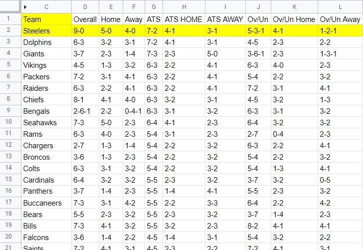
    • Cell C1 - Headers/Column Titles
      • =importxml(A1,A2)
    • Cell C2 - Team names Column
      • =ARRAYFORMULA(trim(transpose(query(transpose(query({importxml(A1,A3)})),,COLUMNS(query({importxml(A1,A3)}))))))
    • Cells D2-L2 (9 columns) - column data
      • Overall: =arrayformula(substitute(ARRAYFORMULA(SUBSTITUTE(trim(transpose(query(transpose(query({importxml(A1,A4)})),,COLUMNS(query({importxml(A1,A4)})))))," "," → "))," → ",""))
      • Home: =arrayformula(substitute(ARRAYFORMULA(SUBSTITUTE(trim(transpose(query(transpose(query({importxml(A1,A5)})),,COLUMNS(query({importxml(A1,A5)})))))," "," → "))," → ",""))
      • Away: =arrayformula(substitute(ARRAYFORMULA( SUBSTITUTE( trim(transpose(query(transpose(query({importxml(A1,A6)})),,COLUMNS(query({importxml(A1,A6)})))))," "," → ") )," → ",""))
      • ATS: =arrayformula(substitute(ARRAYFORMULA( SUBSTITUTE( trim(transpose(query(transpose(query({importxml(A1,A7)})),,COLUMNS(query({importxml(A1,A7)})))))," "," → ") )," → ",""))
      • ATS Home: =arrayformula(substitute(ARRAYFORMULA( SUBSTITUTE( trim(transpose(query(transpose(query({importxml(A1,A8)})),,COLUMNS(query({importxml(A1,A8)})))))," "," → ") )," → ",""))
      • ATS Away: =arrayformula(substitute(ARRAYFORMULA( SUBSTITUTE( trim(transpose(query(transpose(query({importxml(A1,A9)})),,COLUMNS(query({importxml(A1,A9)})))))," "," → ") )," → ",""))
      • Ov/Un: =arrayformula(substitute(ARRAYFORMULA( SUBSTITUTE( trim(transpose(query(transpose(query({importxml(A1,A10)})),,COLUMNS(query({importxml(A1,A10)})))))," "," → ") )," → ",""))
      • Ov/Un Home: =arrayformula(substitute(ARRAYFORMULA( SUBSTITUTE( trim(transpose(query(transpose(query({importxml(A1,A11)})),,COLUMNS(query({importxml(A1,A11)})))))," "," → ") )," → ",""))
      • Ov/Un Away" =arrayformula(substitute(ARRAYFORMULA( SUBSTITUTE( trim(transpose(query(transpose(query({importxml(A1,A12)})),,COLUMNS(query({importxml(A1,A12)})))))," "," → ") )," → ",""))

URL and XPaths

Paths


Output

Highlighted cells indicate a cell containing a formula.

Output


Credit: Max Makhrov: How to use CONCAT in QUERY?

6
  • @Rubén I tried to replicate the inclusion of column() in the Xpath as you did in Trying to use Google Sheets importHTML() to import a table. It forces content to a date format. This would simplify this answer. Needless to say, I didn't manage it ;) Are you able to weave your magic over the Xpath?
    – Tedinoz
    Commented Nov 22, 2020 at 9:34
  • Thank you for the information everyone! Commented Nov 22, 2020 at 23:43
  • 1
    Here is a formula that is better than the one in my previous comment =ArrayFormula(REGEXREPLACE(SPLIT(TRANSPOSE(SPLIT(JOIN("",TRANSPOSE(QUERY(TRANSPOSE({IMPORTXML(A1,"//tr/*"),TRANSPOSE(SPLIT(REPT(REPT("|,",9)&"*,",33),","))}),,1000000))),"*")),"|")," {0,}- {0,}","-")) Commented Nov 23, 2020 at 2:03
  • 1
    @Ruben Stunning. Please do write an answer for this formula. This is infinitely better (more concise, elegant, refined, less complicated/convoluted) than my effort.
    – Tedinoz
    Commented Nov 23, 2020 at 2:13
  • See Tyler's answer Commented Nov 25, 2020 at 14:57
2

@John Tokish, this should do the trick:

=ArrayFormula(REGEXREPLACE(TO_TEXT(IMPORTHTML("https://www.actionnetwork.com/nfl/nfl-against-the-spread-standings","table",1)),"200|20.+$",""))

As you see, I've first converted the entire IMPORT* TO_TEXT. This takes care of everything but the W-L-T formats, which can easily be converted with the REGEXREPLACE, since all W-L-T will come through as text-dates with years in the 2000s.

Of course, if you have the URL in another cell (e.g., A1), the formula can be shortened:

=ArrayFormula(REGEXREPLACE(TO_TEXT(IMPORTHTML(A1,"table",1)),"200|20.+$",""))
2
  • Such simplicity. You replace "200|20.+$"; I understand (I think), the "200" element but would you explain why the "|20" (or 20 ??) is included as well?
    – Tedinoz
    Commented Nov 25, 2020 at 21:45
  • 1
    @Tedinoz, I probably didn't strictly need to include that. But all W-L-T listings are going to try to form a date. Most will translate -1 or -2 as 2001 or 2002. But, theoretically, if one of the elements went over 9, a date year could arbitrarily show up as 2010, 2014, even 2020. Again, not likely. But I ruled it out with that added bit, since it didn't take much formula space to include.
    – Erik Tyler
    Commented Nov 26, 2020 at 0:27
1

Here is a solution using a single formula

=ArrayFormula(
REGEXREPLACE(SPLIT(TRANSPOSE(SPLIT(JOIN("",TRANSPOSE(QUERY(TRANSPOSE(
{IMPORTXML(A1,"//tr/*"),TRANSPOSE(SPLIT(REPT(REPT("|,",9)&"*,",33),","))}
),,1000000))),"*")),"|")," {0,}- {0,}","-")
)

It will only works while the table to imports keeps it's current shape:

  • 9 columns
  • 1 headers row
  • 33 rows, one for each team.

The formula use IMPORTXML instead of IMPORTHTML because it allows us to use xPath.

xPath allows us to select the nodes text to be imported.

It's worthy to note that IMPORTXML doesn't solve that some team stats (wins-loses-draws) be converted to dates but, considering that the wins-loses-draws have a node between them we could import each of these values in separate cells.

In this case IMPORTXML is resturning a an array of values having a single column. TRANSPOSE, QUERY, JOIN, SPLIT, REPT are used to transform the single column into a 34 rows x 9 columns table.

REGEXREPLACE is used to remove the extra spaces by using a regular expression to match the spaces and dash between the wins, loses and draws resulting from IMPORTXML and the xPath used.

Your Answer

By clicking “Post Your Answer”, you agree to our terms of service and acknowledge you have read our privacy policy.

Not the answer you're looking for? Browse other questions tagged or ask your own question.