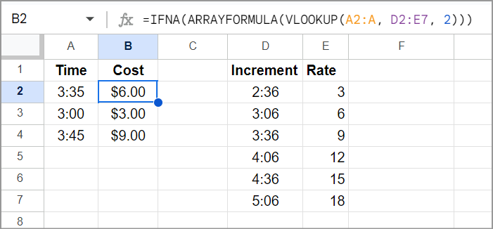
Spoiler
=VLOOKUP(A2, $D$2:$E$7, 2) // Basic
=ARRAYFORMULA(VLOOKUP(A2:A4, D2:E7, 2)) // Array
=IFNA(ARRAYFORMULA(VLOOKUP(A2:A, D2:E7, 2))) // Error Handling
VLOOKUP
This is an excellent candidate for the VLOOKUP function which looks for a value in the first column of a range, then returns the value in the same row, but in the column you specify.
It also supports approximate matches which is great for your needs. If your lookup table is sorted by time (ascending)VLOOKUP will find the largest match that is less than or equal to the lookup value.
Syntax
=VLOOKUP(search_key, range, index, [is_sorted])
Assumptions
All variations assume the following:
D2:E7 is the range containing your lookup table (rate sheet):
D2:D7 contains start times (column 1 of the range)E2:E7 has the rate for each start time (column 2 of the range)
A2:A contains the time(s) you want to checkB2:B contains the formula result(s).
|
A |
B |
C |
D |
E |
F |
| 1 |
Time |
Cost |
|
Increment |
Rate |
|
| 2 |
3:35 |
$ 6.00 |
|
2:36 |
3 |
|
| 3 |
3:00 |
$ 3.00 |
|
3:06 |
6 |
|
| 4 |
3:45 |
$ 9.00 |
|
3:36 |
9 |
|
| 5 |
|
|
|
4:06 |
12 |
|
| 6 |
|
|
|
4:36 |
15 |
|
| 7 |
|
|
|
5:06 |
18 |
|
1. Basic Formula
This is the kind of formula that you copy down into other rows, so the range is absolute to stop it from changing when copied: $D$2:$E$7 vs. D2:E7
=VLOOKUP(A2, $D$2:$E$7, 2)
2. ARRAYFORMULA
The ARRAYFORMULA function enables a single VLOOKUP formula to return the results for multiple rows. The search_key argument is changed to the range A2:A4
=ARRAYFORMULA(VLOOKUP(A2:A4, D2:E7, 2))
3. IFNA
If you wrap the formula in the IFNA function, you don't need to worry about blank rows and can also use an infinite range such as A2:A. Any new rows of times you add would be automatically calculated:
=IFNA(ARRAYFORMULA(VLOOKUP(A2:A, D2:E7, 2)))


