How to use a query with a combination of If and Where

Question

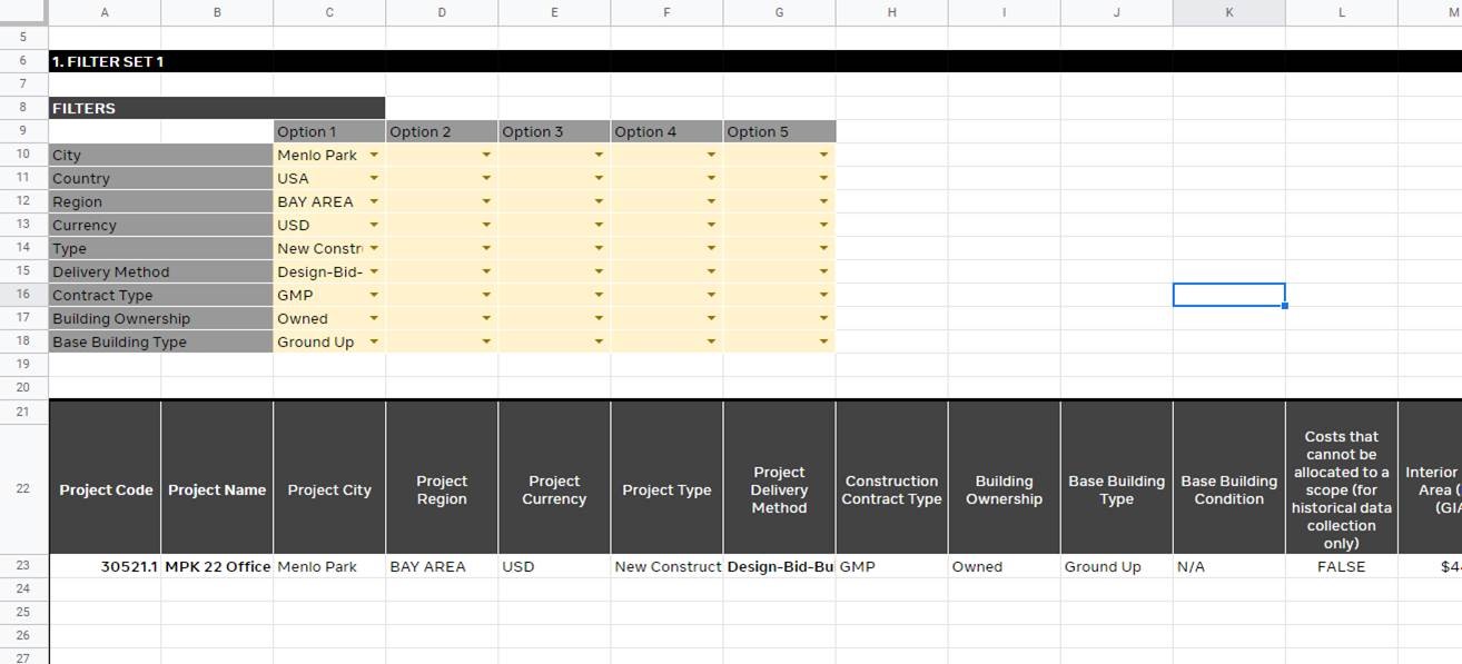
I have a data base on Google sheet. See the spreadsheet at this link:https://docs.google.com/spreadsheets/d/1NGkH56Ga95osN8eBI6d5MhV7SnoEPK4Oe7ymRJVK7M0/edit#gid=1262146092 It s a copy so feel free to make any edit.

I am trying to filter information from the database using a query:

The filters are selected in the cell in yellow line 10 to 18 The query formula is in cell A22 and populates the lines and columns below. I want the formula to return information from the database that matches (L10 Option 1 or L10 Opt 2 …. L10 Opt 5) AND (L11 Opt 1 or.. or.. L11 opt5) AND… and so on until that last line. If “all” is selected in option 1, then it doesn’t filter on that criteria.

The formula below works for all lines, but not if "all" is selected (written only for the 1st 2 lines below):

=query('6. Database'!1:190,"select A,B,D,F,G,H,I,J,K,L,M,AD,BA,CD,CQ,CR,CU,CY,DE,FF,FM,FS where (D = '"&C10&"' or D='"&D10&"' or D='"&E10&"' or D='"&F10&"' or D='"&G10&"') and (E = '"&C11&"' or E='"&D11&"' or E='"&E11&"' or E='"&F11&"' or E='"&G11&"') ")

I tried this but it didnt work (formula parse error): =query('6. Database'!1:190,"select A,B,D,F,G,H,I,J,K,L,M,AD,BA,CD,CQ,CR,CU,CY,DE,FF,FM,FS where ('"C10"'<>'all' and (D = '"&C10&"' or D='"&D10&"' or D='"&E10&"' or D='"&F10&"' or D='"&G10&"')) and ('"c11"'<>'all' and (E = '"&C11&"' or E='"&D11&"' or E='"&E11&"' or E='"&F11&"' or E='"&G11&"')) ")

The formula below work when "all" is selected but only for 1 line: =query('6. Database'!1:190,"select A,B,D,F,G,H,I,J,K,L,M,AD,BA,CD,CQ,CR,CU,CY,DE,FF,FM,FS " & if(C10="all",, "where (D = '"&C10&"' or D='"&D10&"' or D='"&E10&"' or D='"&F10&"' or D='"&G10&"') "))

How can I get it to work with the option to select “all” in any line ?

Answer 1

I think this is easier to do with filter() with criteria consisting of regular expressions than a query() with several separate criteria cells.

Insert a new sheet a name it ColumnData. Get just the columns you are interested in with this formula in cell A1:

=query('6. Database'!A1:SJ, "select A, B, D, F, G, H, I, J, K, L, M, AD, BA, CD, CQ, CR, CU, CY, DE, FF, FM, FS", 2)

Then get the headers with this formula in '1. Project Selection'!A21:

={ ColumnData!A1:V1 }

Fetch the data with this formula in '1. Project Selection'!A22:

=iferror( 
  filter( 
    ColumnData!A2:V, 
    not( 
      mmult( 
        sign(not(iferror( 
          regexmatch( 
            trim(ColumnData!A2:V), 
            "(?i)" & A19:V19 
          ), 
          A19:V19 = "" 
        ))), 
        transpose(sign(column(A19:V19))) 
      ) 
    ) 
  ), 
  "(no matching data)" 
)

Clear rows 23 onward to make room for the results.

You can then write your column-by-column criteria in row 19 as regular expressions like 123|432 or new|improv. If you want to continue using the drop-down lists in A9:G17, you can also use formulas like this (example for cell C19):

=textjoin("|", true, A9:G9)

To learn the exact regular expression syntax used by Google Sheets, see RE2.

See the Elegant search spreadsheet for a working example. Click get your own copy to test it privately. Note that the example uses search() instead of regexmatch().