1

I've googled this various different ways, but haven't found anything that has worked. I have a list that needs to be Private filtered by condition using a custom formula in google sheets.

In Sheet2 I have a list of names with shifts in Column C, in Sheet1 I have a list of shifts that correspond to a day of the week in Column B. I want the private filter to filter out by the list in Sheet1, Column B.

I have used =Regexmatch(C:C,Sheet1!B:B), I have used =Countif(C:C,Sheet1!B:B), I have used =C:C=Sheet1!$B:$B and nothing has worked please help. Thank you

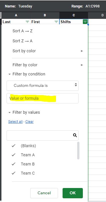
Edited to add: I have included a link to a sample sheet https://docs.google.com/spreadsheets/d/1s_M7U5QwdSF1hEJ_7tPP3_PmfS_OIL27JFbceTGRUzY/edit?usp=sharing First tab has the shifts by day of the week, second tab has names with shifts. Screenshot of the filter view by condition If I create a new filter view and name it Tuesday, I would like the shifts from Tuesday to be automatically be filtered based on the custom formula that pulls from the list in the "Shifts" tab.
5
  • Hi and welcome. The terms that you have used in your question are unclear - specifically a list of names with shifts and list of shifts that correspond to a day of the week. Would you please edit your question to provide some sample data for Sheet1-Column N and Sheet2-Column C, and an example of how a successful outcome would appear.
    – Tedinoz
    Commented Dec 15, 2021 at 4:26
  • @Tedinoz thank you for the feedback, I added a sample sheet and picture
    – Cz713
    Commented Dec 15, 2021 at 14:52
  • So, if I understand you correctly... presently "Tuesday" shows a list of "Shift groups" (Team A, B, C &D). Your goal is to create a list of the names of the people working in those shift groups - that is, create a list of the names of people working on Tuesday. Is that right?
    – Tedinoz
    Commented Dec 15, 2021 at 21:37
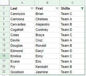
  • I added a sample sheet and picture Your picture shows the Filter menu process. This is not important - what you need to do is show a picture of the outcome of a successful filter. You'll have to create this manually. Hint: don't worry trying to put the filter icons in the header row, just show the header and data that you would expect to see.
    – Tedinoz
    Commented Dec 15, 2021 at 22:48
  • You've written this question with the expectation of using a filter. I wonder whether this is what is known as an X Y problem; that is you've focused on a specific way of solving a problem, rather than describing the problem and being open minded about how it might be solved. For example, I think it likely that the outcome that you want using the method can't be done using the technique that you proscribed BUT it is possible to get that same outcome using other means. Would you access an alternative approach?
    – Tedinoz
    Commented Dec 15, 2021 at 22:57

1 Answer 1

1

You want to "filter" a list of names (with shift groups) based on shift groups.

Option#1 - Filter (menu)

=arrayformula(ifna(match(C2:C22,Shifts!$B$2:$B$5,0),0))>0

  • Filter the "Shifts" column
    • select Filter by Condition
    • select Custom formula
    • enter the formula.

Using match, the formula returns the index value of a match between Shifts (Column C2:C22) and the values in the "Tuesday" column of the "Shifts" sheet (Shifts!$B$2:$B$5). If there is no match, the formula returns a value of zero. By making the condition = >0, the formula will return only those matching values.

This formula has a disadvantage - the filtered day from the Shifts sheet is hard-coded which makes it inconvenient to change.

filter


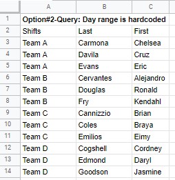
Option#2 - Query: hardcoded 'day'

=query(Names!A1:C22,"select C, A, B where "&"C='"&textjoin("' OR C = '",true,Shifts!B2:B5)&"' order by C",1)

Enter this formula in any sheet, and it will return the same information as the filter option.

  • Note, that filtered day from the Shifts sheet is hard-coded.

query_hardcoded


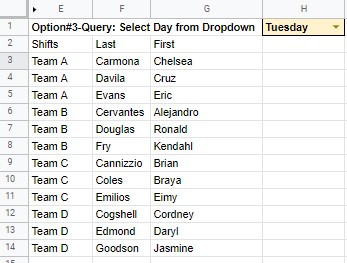
Option#3-Query: Select Day from Dropdown

=query(Names!A1:C22,"select C, A, B where "&"C='"&textjoin("' OR C = '",true,indirect(address(2,match($H$1,Shifts!A1:G1,0),4,true,"Shifts")&":"&address(100,match($H$1,Shifts!A1:G1,0),4)))&"' order by C",1)

  • Enter the formula in any cell
  • Create a Data Validation dropdown (cell H1) by referencing the range =Shifts!$A$1:$G$1.

The formula now references the "day" by matching the dropdown value. This approach makes it easy to modify data reporting.

query_dropdown

Your Answer

By clicking “Post Your Answer”, you agree to our terms of service and acknowledge you have read our privacy policy.

Not the answer you're looking for? Browse other questions tagged or ask your own question.