How to get value of cell by row key and column key

Question

Suppose I have a workbook with two worksheets, data and view. data is structured in "database" style, i.e. with a single header row and unique keys in the first column, e.g.:

Country   GDP  Landlocked
Austria   418   1
France   2770   0
Spain    1480   0

In the view sheet, I wish to look up the data in data by using the column name (i.e. the value of the relevant cell in the header row in data) and the row name (i.e. the value of the relevant cell in the unique key column in data). Here is one way to do this, if I wanted to retrieve, e.g. the GDP value for France:

=vlookup("France",data!$A$1:$YY,match("GDP",data!$1:$1,0),false())

However, this is rather verbose and requires two functions. Are there any more concise ways to achieve the goal?

P.S. If you're wondering why I specified the first range above as data!$A$1:$YY, please see this question.

Answer 1

If you're looking for just the GDP of France then this will do:

=VLOOKUP("France",data!A2:C,2,FALSE)

Answer 2

If you did know the exact column of GDP then Jacob's function would be simpler.

If you do not know the exact column of GDP or row of France, then your function actually works quite well. You could also use Index(Match()) like this:

=index(data!$A$2:$YY;match("France",$A$2:$A,0);match("GDP",$A$1:$YY,0))

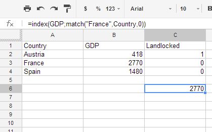
You can also name each column in 'Data'->'Named and Protected Ranges'. IE. the Name "GDP" would reference "data!B2:B". This would allow you to do the following:

=index(GDP;match("France",Country,0))

This is very useful when using drop down menus or data validation. You can use the Indirect() function to automatically populate a drop down with choices based off a user input or other drop down menu.