0

I have a Auction that I am updating and posting bids to on a Google Sheet that bidders can view. The condition to the auction is that the item will be sold to a bidder if no one has bid on said item within 24 hours, thus closing the auction.

I have the sheet to update the time edited for a row whenever I alter the current offer for an item, as well as posting a deadline for bidding on said item to 24 hours after the last alteration.

Example of Sheet Structure

With that in mind, I am trying to use Conditional Formatting to highlight the Deadline cell whenever the current Real Time clock is within 1 hour of the deadline. I have tried multiple formulas with other StackExchange answers as my base, as well as what I believe should work fundamentally with no avail.

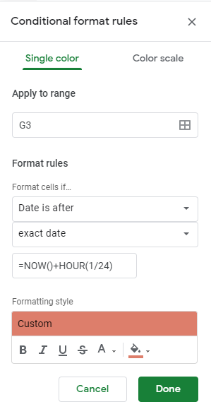
Formula example 1/? enter image description here

With the above example I would expect to see cell G3 to highlight red at 18:00. But through testing found that it doesn't apply.

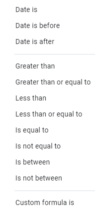
I have also tried formulas that read both the last time edited and the deadline to create formatting conditions based on a comparison of the cells data to the formula. Such as below, attempting each and other variations on the same idea with each "if" in the 3rd image.

=G3-HOUR(1/24)
=G3-TIME(1,0,0)
=F3+HOUR(23/24)
=F3+TIME(23,0,0)

Any assistance to get this to work would be greatly appreciated. I had hoped that I could simply alter the post answers below but they don't seem to apply to an hourly basis.

Stack Exchange Post #1

Stack Exchange Post #2

Stack Exchange Post #3

Once Again, any assistance is greatly appreciated. If possible along with the solution, could I also get an explanation of where my thought process faltered.

2 Answers 2

1

Try this:

Set the "Apply to Range" field to G3:G (assuming you will have items and times in multiple rows).

Set "Format cells if" to Custom formula is.

In the formula field below that, enter this formula: =G3 > NOW() - 1/24

Set the "Formatting style" section as you like.

Click Done.

4
  • Thank you so much for this, It didn't quite work how I intended to convey through my post, but with very slight testing and modifications, I used your formula as a basis for the final iteration I'll be using. I will also post the Answer to my own question with the final formula soon. Commented Aug 11, 2021 at 3:57
  • You may have wanted =(G3 - NOW()) < 1/24
    – Erik Tyler
    Commented Aug 11, 2021 at 3:59
  • It is always a bit tricky to write formulas for a sheet we can't see. I'm glad I could point you in the right direction. At the end of the day, the problem is solved. That is the important thing.
    – Erik Tyler
    Commented Aug 11, 2021 at 4:00
  • Once again thank you for the assistance, your post was extremely insightful, I wish I wasn't so new to StackExchange, otherwise, I would cast a vote for your answer to show how much it helped achieve a suitable solution. Commented Aug 11, 2021 at 4:47
0

Thanks to the assistance of Erik Tyler and his work below, I was pointed towards a simple solution for my use case.

Try this:

Set the "Apply to Range" field to G3:G (assuming you will have items and times in multiple rows).

Set "Format cells if" to Custom formula is.

In the formula field below that, enter this formula: =G3 > NOW() - 1/24

Set the "Formatting style" section as you like.

Click Done.

The only changes made to the formula presented above was a change to how the formula targets cells by altering the target of G3 in the example to G:G as a failsafe to make sure the Conditional Format is applied to all cells in the column correctly.

The secondary change is the direction that the time is of the cell is compared, in which the "greater than" is substituted for "less than" and the "minus" being replaced by a "plus" as well, Giving us a final formula of; =G:G < NOW() + 1/24.

Just to finally reiterate for anyone else who may need this specific solution.

  1. Set the "Apply to Range" field to the column letter you want the format to apply to, the first row number, colon, then the same column letter (which assumes you want the rest of the column highlighted)

    E.g - A#:A

  2. Set "Format cells if" to Custom formula is.

  3. In the formula field below that, enter the formula in this format: =A:A < NOW() + 1/24

  4. Set the "Formatting style" section as you like.

  5. Click Done.

This will update the cell as soon as it is 1 hour before the time posted within the cell. This is useful for deadlines in school curriculum, baking times, auctioning and so forth.

If you are also in a use case such as auctioning where multiple people are viewing the sheet, I would suggest updating the recalculation to "On change and every minute" to ensure that the cell formatting is time accurate for the viewer

I would also look at the comments on each answer to view possible alternative solutions.

Your Answer

By clicking “Post Your Answer”, you agree to our terms of service and acknowledge you have read our privacy policy.

Not the answer you're looking for? Browse other questions tagged or ask your own question.