Return value by lookup from multiple value

Question

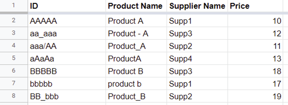
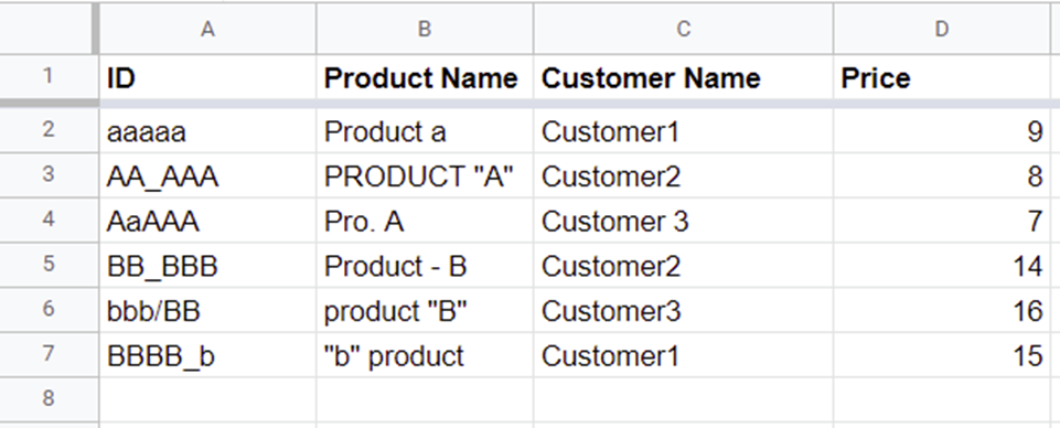
We constantly receive offers from suppliers and requests from customers. The problem is that customers and suppliers usually have several different identifiers for the same product. Like this:

customer requests

supplier offers

In order see the matches between the offers and requests, I need to create a sheet with the unique products with the Product Name and Main ID we want to use. Next to the Main IDs, I need to enter all the alternative IDs that I met in offers and requests. Something like this:

product_data

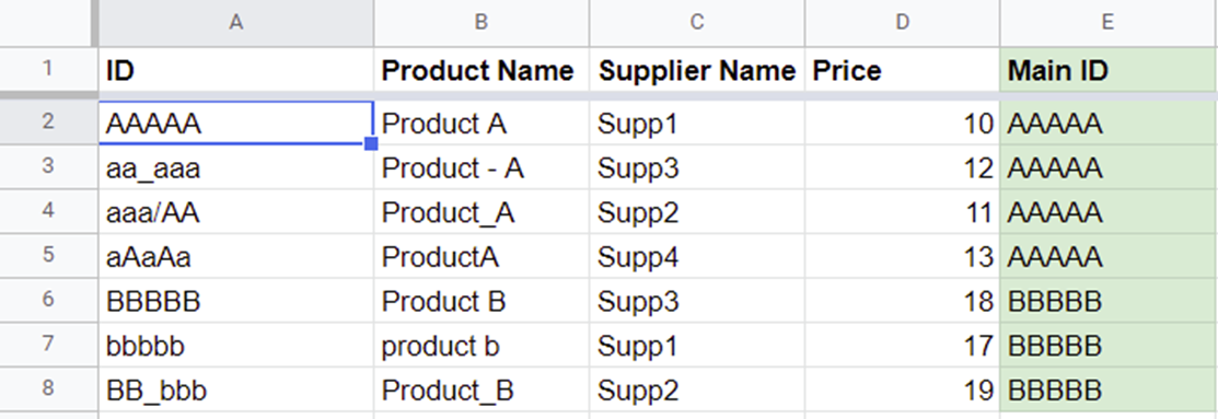
My question is what is the best formula to make google sheet look for the IDs in offers/requests from column C to column I of product_data sheet (from ALT ID 1 to ALT ID 7 )and based on that, return the MAIN ID of the product in offers/request? like this:

Answer 1

Try this:

=QUERY(
    'ID-LookUp'!$A$2:$I$3,
    "SELECT B WHERE " &
    REGEXREPLACE(
        CONCATENATE(
            ArrayFormula(
                SPLIT(
                    "B,C,D,E,F,G,H,I",
                    ","
                ) & " = " &
                CHAR(
                    34
                ) & A2 &
                CHAR(
                    34
                ) & " OR "
            )
        ),
        "OR $",
        ""
    ),
    0
)

Explanation

Alright the REGEXREPLACE thing first. We are basically first generating the WHERE clause for the QUERY function there. we take the array which just has B through I then append to each = "ID" OR. The ID part we get from the A column. We then use REGEXREPLACE to remove the redundant "OR" at the end.

We move now to the main QUERY function. We select the data only (A2:I3 not A1:I3). This is to make sure that the header doesn't show up. Next we select B since it contains the Main ID we want to return. We then append the string and done.