1

I need help, I want to combine multiple cells in one other cell in another sheet.
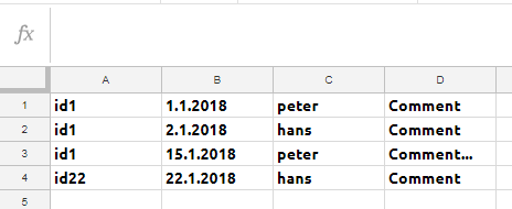
I have 4 Collums in my first Sheet1, filed with data:

  1. Id's (A1:A)
  2. Dates(B1:B)
  3. Name(C1:C)
  4. Comments(D1:D)

And on my other Sheet2, I can select Id's(G3) from a dropdown and get more data from other sheets. Now I want to Combine all Dates, Name and Comment in one cell on my Sheet2.
I want something like, I pick an Id on Sheet2 and get every Comment with name and Date from Sheet1 in one cell.
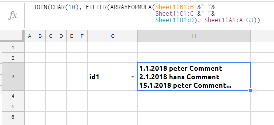
I want it like

1.1.2018 peter Comment  
2.1.2018 hans Comment  
15.1.2018 peter Comment...

The cell can expand I only need everything in one cell.
Is that possible and how?

3 Answers 3

0

if you need it everything in one cell, try this:

=JOIN(CHAR(10); FILTER(ARRAYFORMULA(Sheet1!B1:B &" "&
                                    Sheet1!C1:C &" "&
                                    Sheet1!D1:D); Sheet1!A1:A=G3))


blank error fix:

=IF(G3<>""; JOIN(CHAR(10); FILTER(ARRAYFORMULA(Sheet1!B1:B &" "&
                                               Sheet1!C1:C &" "&
                                               Sheet1!D1:D); Sheet1!A1:A=G3));)

3
  • Thanks a lot, now another question how can I insert a line break or an empty line after every line?
    – Vic
    Commented Sep 3, 2018 at 16:27
  • @Vic add one more CHAR(10)
    – user0
    Commented Sep 3, 2018 at 22:14
  • @Vic =JOIN(CHAR(10); FILTER(ARRAYFORMULA(Sheet1!B1:B &" "& Sheet1!C1:C &" "& Sheet1!D1:D&CHAR(10)); Sheet1!A1:A=G3))
    – user0
    Commented Sep 3, 2018 at 23:11
0

If you're using a drop down this should work

=TEXTJOIN(",", True,QUERY(A:D, "Select * Where A = '"&E2&"' ",0))

you will need to change your query to match ur data. share a copy of ur sheet if u can.

2
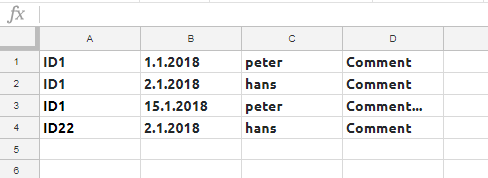
  • i.sstatic.net/t5oBL.png this won't do as OP requested to be formatted
    – user0
    Commented Aug 30, 2018 at 7:39
  • Yes, you're correct. your solution is much more elegant. I would make this a two step solution. One to query the drop down two to write a formula down the adjacent column with text joins so each record appears on a new line.
    – Umar.H
    Commented Aug 30, 2018 at 8:10
0

you need this in Sheet2!H3:

=FILTER(ARRAYFORMULA(Sheet1!B1:B&" "&Sheet1!C1:C&" "&Sheet1!D1:D); Sheet1!A1:A=G3)


#N/A fix:

=IFERROR(FILTER(ARRAYFORMULA(Sheet1!B1:B&" "&Sheet1!C1:C&" "&Sheet1!D1:D);Sheet1!A1:A=G3);)

Your Answer

By clicking “Post Your Answer”, you agree to our terms of service and acknowledge you have read our privacy policy.

Not the answer you're looking for? Browse other questions tagged or ask your own question.