1

Say I have a list of dates in column A, many of them are multiple entries. The dates are sorted and currently in time-stamp form (text).

I want to alternate the cell color of the data in the columns next to the dates every time the date in column A changes to make the data from different dates stand out.

Is there a way to do this in Google Sheets?

Thanks

5
  • 3
  • @Rubén After reading the linked question and answers, the answer to OP's question did not become obvious to me.
    – user135384
    Commented Feb 25, 2018 at 4:42
  • @FTP Have you tried the Google Sheets built-in conditional formatting feature? Commented Feb 25, 2018 at 4:54
  • I did not see a way to accomplish this in the formatting tool. I don't know what the values will be, not all dates will exist, and there will be different numbers of those that do exist. All I do know is that there will be different dates, and I want to set those apart with alternating color. Also, the range to be formatted will be expanding as new dates are added.
    – Steve
    Commented Feb 25, 2018 at 19:33
  • Can you include a minimal example of what you are trying to achieve? I have a few solutions in mind. But your scenario seems a bit convoluted.
    – Argyll
    Commented Mar 4, 2018 at 2:48

1 Answer 1

2

I'm not sure I understood your question... But here is one possible answer:

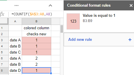
You can apply the formula COUNTIF to the next column like this: enter image description here

The beginning of the interval will be fixed and the end will be increasing, while you push the formula down to new cells.

So, the fist time a date appears, the content of the cell will be "1". You can then format conditionally the cell for a specific format when it is "1".

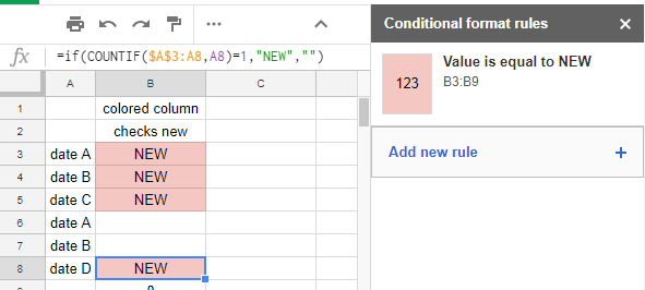
If you don't like to see numbers, you can apply the function IF to get a more user friendly look to your file and adapt the conditional format accordingly : enter image description here

Does this help?

3
  • Interesting - but no. I am not just looking for the first occurrence of a date - they are sorted anyway. But that might be a partial solution.
    – Steve
    Commented Feb 28, 2018 at 4:59
  • That might be close to a partial solution. By checking to see if the date value is different than the one above it and returning a 1 if it is, you can then sum those 1s and check for an odd or even condition to then set the color based on known possibilities rather than on unknown dates. Now just need to spread that across each row individually and make sure it can be expanded as new dates are added.
    – Steve
    Commented Feb 28, 2018 at 5:31
  • @Steve I'm sorry, but I still don't understand what you need. You wish to paint the next cell of the same dates with the same color? That is, every time date A shows up, the next cell will be green; every time date B shows up, the next cell will be red; and so on?
    – Ceu Melo
    Commented Feb 28, 2018 at 9:29

Your Answer

By clicking “Post Your Answer”, you agree to our terms of service and acknowledge you have read our privacy policy.

Not the answer you're looking for? Browse other questions tagged or ask your own question.