Conditional formatting formula to highlight duplicates but only if the date equals today

Question

I'm trying to write a conditional formatting rule to highlight cells in B3:B that are duplicates, but only if today's date is in column A.

I started with =COUNTIF(B3:B,B3)>1 which returned the duplicate values, but I have tried to add a COUNTIFS or a TODAY condition and nothing seems to work.

countifs(A3,:A"<="TODAY(),(B3:B,B3)>1

Answer 1

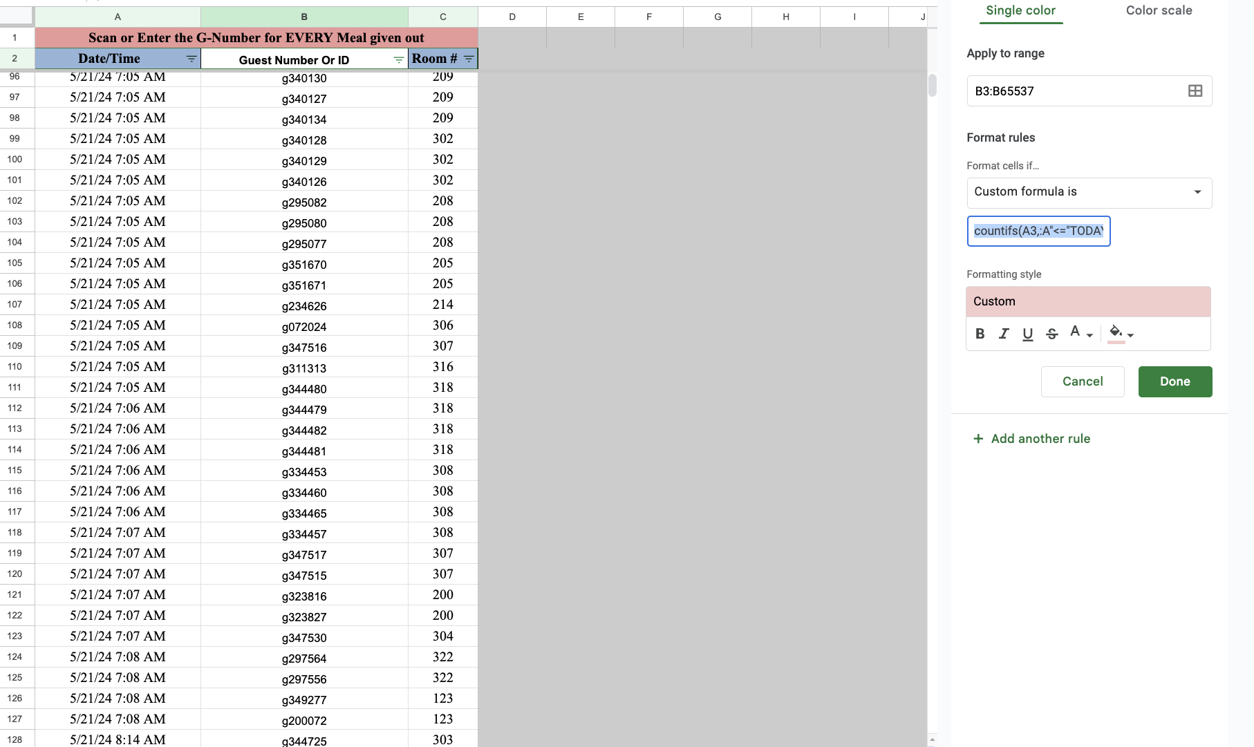
TL:DR

=AND(INT(A3)=TODAY(), SUMPRODUCT(INT($A$3:$A)=TODAY(), $B$3:$B=B3)>1)

Exclude Time

You need to remove the times, (fractions of days) from the dates when comparing to TODAY. The INT function will return the integer portion of a number.

=VALUE("05/23/2024") <> VALUE("05/23/2024 1:15 PM") 
=VALUE("05/23/2024") = INT("05/23/2024 1:15 PM")

Formula

The SUMPRODUCT function is well-suited to your use case:

=AND(INT(A3)=TODAY(), SUMPRODUCT(INT($A$3:$A)=TODAY(), $B$3:$B=B3)>1)

Equivalent:

=((INT(A3)=TODAY())*(SUMPRODUCT(INT($A$3:$A)=TODAY(), $B$3:$B=B3)>1))

Explanation

1. The first test is to check if the current row of Column A, A3 in the example, includes today's date. INT is used to remove any time from A3 (returns only integers).

   INT(A3)=TODAY()
   

2. The next test uses SUMPRODUCT, an array formula, to return the sum of columns multiplied together.

   SUMPRODUCT(INT($A$3:$A)=TODAY(), $B$3:$B=B3)>1
   

   1. The first column, is created by testing each row in Column A for today's date. The resulting column of TRUE and FALSE are interpreted as a column of 1 and 0 in the function.

      INT($A$3:$A)=TODAY()
      

   2. The second column is created by testing each row in Column B to see if it is equivalent to the current row's value, B3 in the example. The resulting column is also interpreted as 1 and 0 values.

      $B$3:$B=B3
      

   3. When the two columns are multiplied together in the array formula, rows where both columns passed their test return 1 and rows where any column failed return 0.

      Col1	Col2	Col1 * Col2
      1	1	1
      1	0	0
      0	1	0
      0	0	0

   4. SUMPRODUCT adds up the product and if the result is greater than 1, it indicates there were multiple rows with both today's date and the same value in Column B

Empty cells in Column B

If you have multiple rows with today's date but where Column B is empty and you don't want them highlighted, the formula should be modified to check if Column B in the current row is empty LEN(B3) or B3<>""

=AND(LEN(B3), INT(A3)=TODAY(), SUMPRODUCT(INT($A$3:$A)=TODAY(), $B$3:$B=B3)>1)

Equivalent:

=LEN(B3)*(INT(A3)=TODAY())*(SUMPRODUCT(INT($A$3:$A)=TODAY(), $B$3:$B=B3)>1)